Anomaly detection in industrial IoT data using Google Vertex AI: A reference notebook

Modern manufacturing, transportation, and energy companies routinely operate thousands of machines and perform hundreds of quality checks at different stages of their production and distribution processes. Industrial sensors and IoT devices enable these companies to collect comprehensive real-time metrics across equipment, vehicles, and produced parts, but the analysis of such data streams is a challenging task.

In this blog post, we focus on IoT data analysis challenges associated with system health monitoring and how to resolve them. Our main goal is to create an analytical pipeline that:

• analyzes IoT metrics collected from some physical system;
• evaluates the probability that the system is in an anomalous state (as opposed to a normal state); and
• makes binary decisions that can be used to trigger automatic actions or alert operations teams to become involved.

We start with a discussion of how the health monitoring problem can be converted into standard machine learning tasks and what pitfalls one should be aware of, and then implement a reference Vertex AI pipeline for anomaly detection. This pipeline can be viewed as a starter kit for quick prototyping of IoT anomaly detection solutions that can be further customized and extended to create production-grade platforms.

Anomaly detection vs system health evaluation

Anomaly detection is a classic problem in statistics, and many off-the-shelf anomaly detection models are readily available. Does this mean that any system health monitoring problem can be straightforwardly solved by applying some standard anomaly detection algorithm to the observed IoT metrics? To answer this question, let us consider a model example that highlights the differences between statistical anomalies (also referred to as outliers) and anomalies that are meaningful from the operational standpoint.

Assume that our goal is to develop a leak detection model for a tank car loading station at a chemical plant, as shown in the figure below. The loading station pumps some liquid chemical from the ground tank to car tanks over a pipe, and we collect measurements from two volume meters installed on the opposite sides of the pipe. At each time interval, we observe a pair of values $(x_{1}, x_{2})$ that can be plotted as shown in subfigure (a). Ideally, the measurements from two meters should be identical, but the actual values can vary depending on pump mode, tank car type, and other factors that we consider to be unknown. The discrepancy between the two measurements indicates the leak.

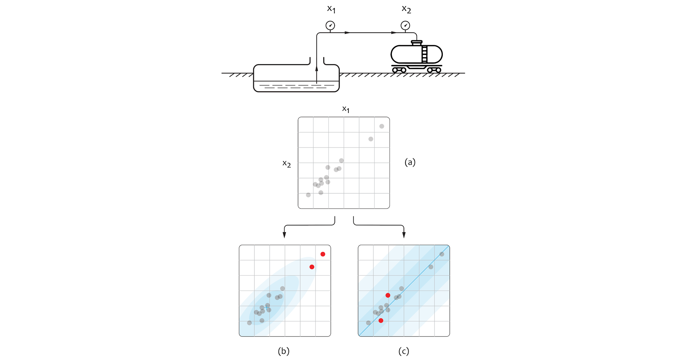
Let’s imagine figure (a) represents the values we observed on our sensors over time. Without understanding the operation of the tank car loading station pump, it is possible to build several very different (yet equally correct) anomaly detection models. These models are illustrated as examples (b) and (c) where red dots indicate anomaly values. For example, we can make an assumption that the points are drawn from the bivariate gaussian distribution, and fit the corresponding model as shown in subfigure (b). This results in scoring the high-volume and low-volume points as anomalous which does not make sense in the context of the environment we have defined. The alternative solution is to build a model that scores the observed samples based on the difference between the metrics, represented as $|x_{1} - x_{2}|$, as shown in subfigure (c). This approach clearly makes more sense because such a model is aligned with the semantics of the data and laws that govern the real-world environment.

This basic example illustrates some of the pitfalls associated with the development of anomaly detection models. First, it demonstrates that it is important to state the semantic definition of anomaly before attempting to classify values as anomalous. Second, it highlights that external factors that impact the system, and our ability to measure or control them, can be critically important for building a valid anomaly detection model. We refine this idea in the next section and tie the anomaly detection problem to standard ML components such as regression and time series forecasting.

Anomaly detection using standard building blocks

In most industrial applications, IoT data comes as a multivariate time series. For example, an engine can be equipped with multiple sensors that measure rotation speed, vibration (acceleration) along several axes, and temperature every 10 seconds. This way, every observation is a vector of metrics that represents the state of the system at a certain point of time.

In some environments, we might have access to labeled data where individual states are marked as either normal or anomalous. However, it is very common to have only the data that correspond to the normal state of the system or have very few anomalous instances that can be sufficient for model evaluation, but not for training. Delving deeper into these scenarios, next we discuss the model design options for when the data does not contain any labeled anomalies, and then review the options for the two-class scenario, when there is a substantial sample of data points labeled as anomalous. The first case is commonly referred to as one-class supervised learning (i.e. the only class available is normal data), and the second case is an example of two-class supervised learning (with normal data and anomalous data classes). We also discuss the difference between treating the observed metrics as independent and identically distributed (i.i.d.) data using regression or classification models and non-i.i.d. data using time series methods.

As a side note, it is worth mentioning that more specialized anomaly detection methods such as clustering and autoencoders can learn in an unsupervised way from a mix of normal and anomalous instances, and semi-supervised methods can learn from highly imbalanced labeled datasets [1, 2]. These methods are beyond the scope of this blog post, however, because we are focusing on how the anomaly detection problem can be solved using only the basic AutoML components.

One-class learning using forecasting models

Assuming that we have only the samples collected from the normally functioning system, we can build a model of normality that captures the regular metric patterns within individual states, as well as the evolution of the states over time. The model of normality can be used to predict the future state of the system, and anomaly scoring can then be performed by comparing the actually observed states with this prediction. If the observed value is very different from the one we forecasted based on historical data, it is deemed an anomaly. If it’s close to the forecasted value then it’s not.

This concept can be naturally implemented using a time series forecasting model (e.g. Vertex AI Forecast). Assuming that we observe a sequence of state vectors $(x_{1}, x_{2}, …)$, we can train a model that estimates the future state $x_{t+1}^{*}$ based on the context $(x_{t}, x_{t-1}, …)$:

$x_{t+1}^{*} = f(x_{t}, x_{t-1}, x_{t-2}, …)$

We can also include additional covariates known at the time moment $t+1$. The anomaly score can then be produced by evaluating the distance between the estimate $x_{t+1}$ and observed state $x_{t+1}$. For example, we can use the mean squared error (MSE) as the measure of distance:

$anomaly\_score = MSE(x_{t+1}, x_{t+1})$

This design is illustrated in the following figure:

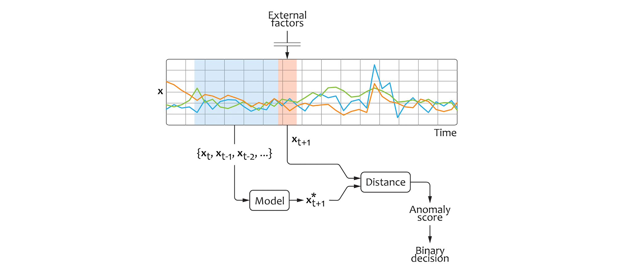
The final binary decision can be made by comparing the anomaly score with a threshold that is optimized to achieve the desirable tradeoff between the false positive and false negative rates. In particular, we can do this by backtesting different threshold values on historical data if some labeled instances are available.

The alternative approach is to estimate the interval (region) where the state is expected to be, and flag the observed state as an anomaly if it falls outside of this interval. For example, we can estimate 5-th and 95-th percentiles for each component of $x_{t+1}$, and deem all states that fall outside of this region as anomalous.

The forecasting approach assumes that the future system state is predictable based on the context, and possibly, additional covariates available at the time of forecasting. This approach works well for rotating machinery (such as compressors, pumps, and turbines), heating and melting processes, and other dynamical systems. However, as we discussed in the previous section, it might not be appropriate for systems that are impacted by unobserved external factors.

One-class learning using regression models

In some environments, we are not able to accurately model the dynamics of the system. For example, let us assume that we are collecting data from accelerators installed in an office building elevator. Although we can assess any particular observation as normal or anomalous depending on the level of vibration, the future vibration levels depend on unpredictable external factors (e.g. whether somebody pushes the call button or not). In this situation we would use a regression model instead of a forecasting model, but the intuition is unchanged. If the observed value is very different from the one produced by the regression model the datapoint is deemed an anomaly.

If we are not able to model the dynamics of the system, we can attempt to learn the manifold of individual states. One possible way to implement this idea is to build a regression model that predicts some components of the state based on the other components. For example, let’s assume the level of vibration (acceleration) in some engine is a function of the rotation speed and torque. We can build a regression model that uses rotation speed and torque as covariates to estimate the acceleration values. This approach makes sense in many practical settings because we can naturally separate the metrics we want to monitor from the covariates.

In a general case, we can formulate the model design as follows:

$x_{t,k}^{*} = f(x_{t,1}, x_{t,2}, ..., x_{t,k-1})$

Here, $x_{t,1}, ..., x_{t,k-1}$ are the covariates and $x_{t,k}$ is the metric we choose to monitor (diagnostic metric). We can now use any model architecture suited for regression problems, for example, by using one of the pre-built pipelines in Vertex AI Tabular Workflows. Similar to the forecasting approach, the anomaly scores can be produced using some distance measure such as MSE and then converted to the binary decision using thresholding:

$anomaly\_score = MSE(x_{t,k}^{*}, x_{t,k})$

We can summarize this design as follows:

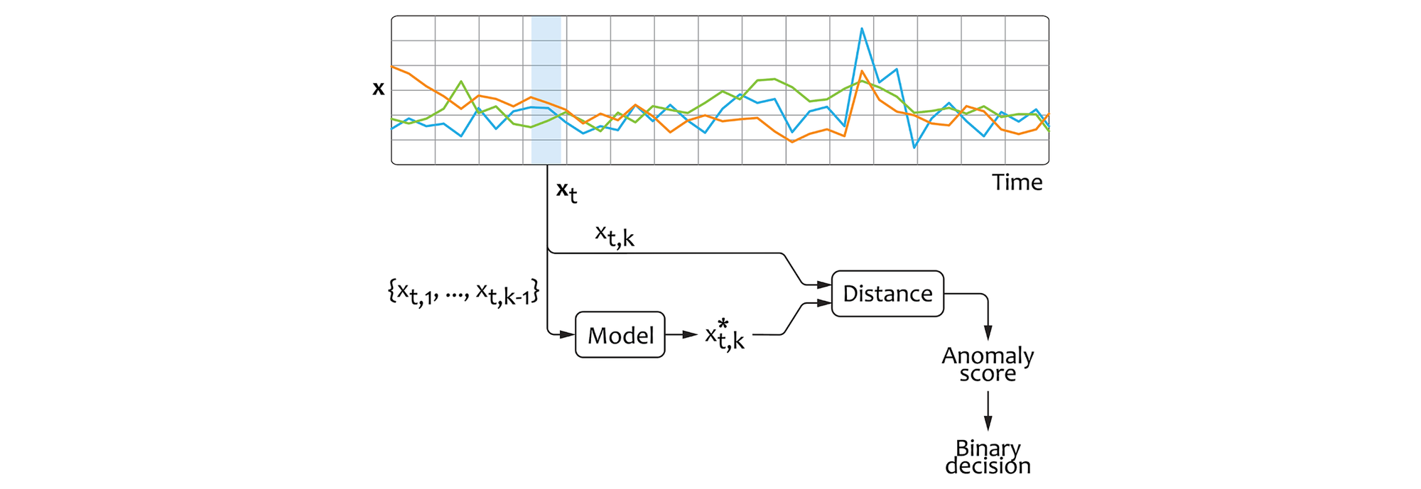
One of the main benefits of the regression approach is that we can choose the limited number of covariates for each diagnostic metric based on our domain knowledge. This helps to reduce the dimensionality of the ML problem in environments with a large number of metrics.

The regression approach is closely related to autoencoding, another popular method for anomaly detection. In autoencoders, we do not delineate between the monitored metrics and covariates, but rather reconstruct all components of the state vector using a limited-capacity model.

Two-class learning using classification models

The third option we can consider is a classification model. Assuming that we have a dataset where the state instances are explicitly marked as normal and anomalous, we can train a classification model that directly estimates the probability of a given state to be normal/anomalous, as displayed in the figure below:

The classification approach not only requires the training data to be labeled, but also entails that the training dataset must contain a sufficiently large number of anomalous instances that cover the entire space of possible anomalies (anomalous manifold). These requirements can be difficult to guarantee in many real-world environments.

Environment and dataset

In this section, we start to develop a reference pipeline for anomaly detection. To build this pipeline, we use an example model of a factory that operates multiple electric motors. We assume that each motor is equipped with multiple sensors, where one measures the metric we want to monitor, and the others measure the parameters that can be interpreted as covariates. This setup is shown in the figure below where we denote the number of motors as m and number of sensor types as k, so that each motor generates a k-variate time series:

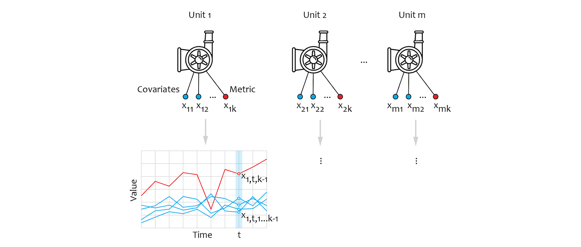
We assume three sensor types: rotation speed, torque, and vibration amplitude. We interpret the rotation speed and torque as covariates that can change in unpredictable ways (e.g. motors can be controlled by a software job or human operator). The vibration amplitude is interpreted as a diagnostic metric that needs to be monitored, but the normal level of vibration depends on the covariates. For example, a certain level of vibration can be normal at high rotation speeds, but indicate a bearing failure if observed at a low speed.

We start with building a simulator of the above environment and generate a synthetic dataset for model training and evaluation. We define a unique function $f_{i}$ for each motor that relates its vibration level $x_{i,3}$ with covariates, where rotation speed is $x_{i,1}$ and torque is $x_{i,2}$. These functions can be viewed as mathematical models of the physical systems. Two examples of such functions are presented in the following figure:

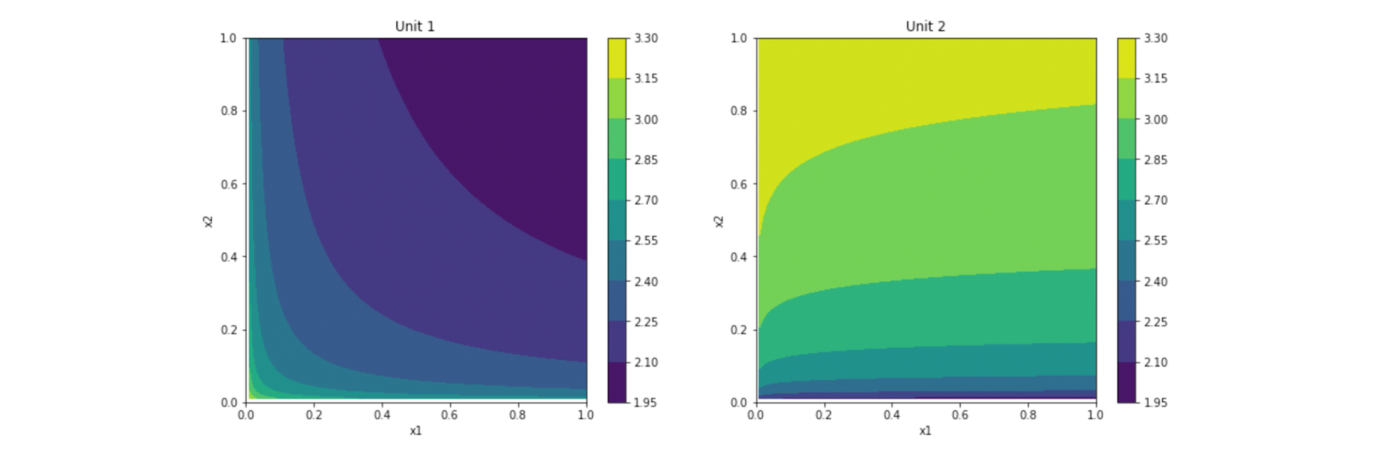
To generate the dataset, we iterate over time steps $t$, draw covariates $x_{t,i,1}$ and $x_{t,i,2}$ from some random distribution for each motor $1 ≤ i ≤ m$ at each time step, and compute the vibration metric $x_{t,i,3}$ as:

$x_{t,i,3} = f_{i}(x_{t,i,1}, x_{t,i,2}) + noise_{t,i}$

The resulting dataset thus has a simple schema that includes the timestamp, motor ID, sensor type, and measured value:

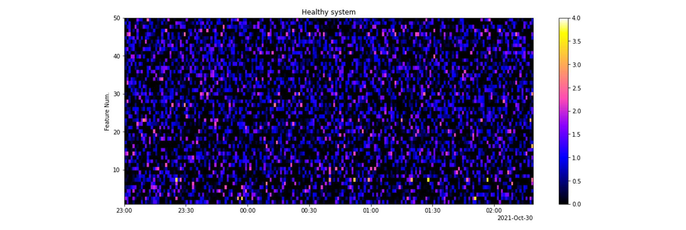
We assume $m=50$ motors and $T=200$ timesteps in total, so we can visualize the generated data for each sensor type as a $50 \times 200$ real-valued matrix. For example, the vibration data for an all-healthy factory is visualized as follows:

Anomaly scoring using an AutoML Regression model

Vertex AI provides AutoML Forecast, Regression, and Classification services which enable us to implement all three approaches described in the previous sections. In this section, we focus on the regression-based approach, but the forecasting-based solution can be implemented in a very similar way. We start with training the regression model on healthy data, then compute the distance between the observed diagnostic metric values and the normal manifold, and then convert the metric into an anomaly score.

We start with training a regression model for each motor. Each such model learns the shape of the dependency between the vibration amplitude $x_{i,3}$ of the i-th motor (our primary diagnostic metric) and covariates that affect the vibration level, where rotation speed is $x_{i,1}$ and torque is $x_{i,2}$. The model selection is not critical here. We normally use a standard neural network, but other options such as regression trees would be a reasonable choice. It is essential that we train the model only on the data collected from a healthy system. Each trained model could be viewed as a function $f_{i}^{*}(x_{i,1}, x_{i,2})$ which is our estimate (approximation) of the unknown $f_{i}(x_{i,1}, x_{i,2})$. In our implementation, we choose to build a single model that takes motor ID as an input categorical feature to simplify the model development and maintenance (as opposed to building 50 separate models). This is the recommended approach unless the covariates/machines are very different.

The next step is to transform the primary diagnostic metric (the vibration amplitude) into the secondary metric that quantifies the deviation from the normal manifold. For each newly arrived sample, we calculate the ratio between the observed and predicted values:

$z_{i} = x_{i,3} / f_{i}^{*}(x_{t,1}, x_{t,2}), \ \ \ for\ i=1,..,k$

We omit the time index, t, here because all values in the above expression correspond to the same moment of time. The dataframe that includes the primary metric (vibration_rms), predicted primary metric (vibration_pred), and secondary metrics (z) looks as follows:

There is an essential distinction between statistical properties of the primary diagnostic metric $x_{i,3}$ (vibration amplitude) and secondary metric $z_{i}$: the latter has much lower variability. This is the case as long as our model is capable of predicting the vibration amplitude from the two covariates. If, for example, the model makes predictions with a very low error, then, for a healthy motor, $z_{i}$ takes values very close to $1.0$, even when the vibration amplitudes $x_{t,i,3}$ vary by orders of magnitude due to changes in the covariates. This property of the secondary metric enables reliable anomaly detection.

When the vibration amplitude is abnormally high, the values of the secondary metric $z_{i}$ tend to be significantly higher than $1.0$. However, the variability of secondary metric $z_{i}$ around the unit value may vary depending on the intrinsic properties and operational conditions of particular motors in their healthy state. For example, the motors for which a healthy vibration amplitude can be predicted with smaller error would tend to have lower variability of $z_{i}$. This suggests that our secondary metric might not be used directly as a reliable anomaly score. Therefore, we apply an additional adaptive standardization to transform secondary metric $z_{i}$ into a useful anomaly score $s_{i}$. The adaptive standardization operation is quite straightforward:

$s_{i} = (z_{i} - mean(z_{i})) / std(z_{i}), \ \ \ for\ i=1,..,k$

Here, $mean(z_{i})$ and $std(z_{i})$ are the mean and the standard deviation of $z_{i}$, calculated on the data from a healthy system. If the distribution of $z_{i}$ has long tails, then one might replace the mean and standard deviation by some robust measure of the location and scale. Such robust statistics are much less sensitive to rare, extremely large values, as compared to the mean and standard deviation. A simple example of such robust measures of location and scale are the median and sum of absolute deviations from the median, respectively. In our experience, many variables in real industrial systems quite often exhibit such long-tail behavior and, thus, robust statistics are preferable.

In a healthy system, the anomaly scores $s_{i}$ tend to vary around zero value within the range of 3-4 units, irrespective of the variability of secondary metrics $z_{i}$. If the vibration level is anomalously high, then anomaly scores $s_{i}$ take much higher values, say, 10-20 and higher. We illustrate the properties of the anomaly scores $s_{i}$ using the synthetic dataset described in the previous section.

First, we train the Vertex AI AutoML Tabular Regression model on the data generated for a healthy system. This step is almost completely automated in Vertex AI. This sharply reduces the effort needed for data preprocessing, model design, optimization of hyperparameters, and evaluation of the optimized model.

Second, we compute anomaly scores $s_{i}$ as described above for another generated dataset where two motors out of 50 gradually develop an abnormal vibration. For a fair comparison, we also perform the adaptive standardization for primary metric $x_{i,3}$.

The standardized primary metric $x_{i,3}$ and anomaly score $s_{i}$ are visualized in the figure below. The values are shown for 50 motors (vertical axis) and 200 consecutive time steps (horizontal axis). The color coding corresponds to the vibration amplitude. There are two anomalies in the 10th and 30th motors. Both anomalies start at 23:10 and gradually increase up to the end of the time interval. The anomaly in the 10th motor is much stronger than the anomaly in the 30th motor.

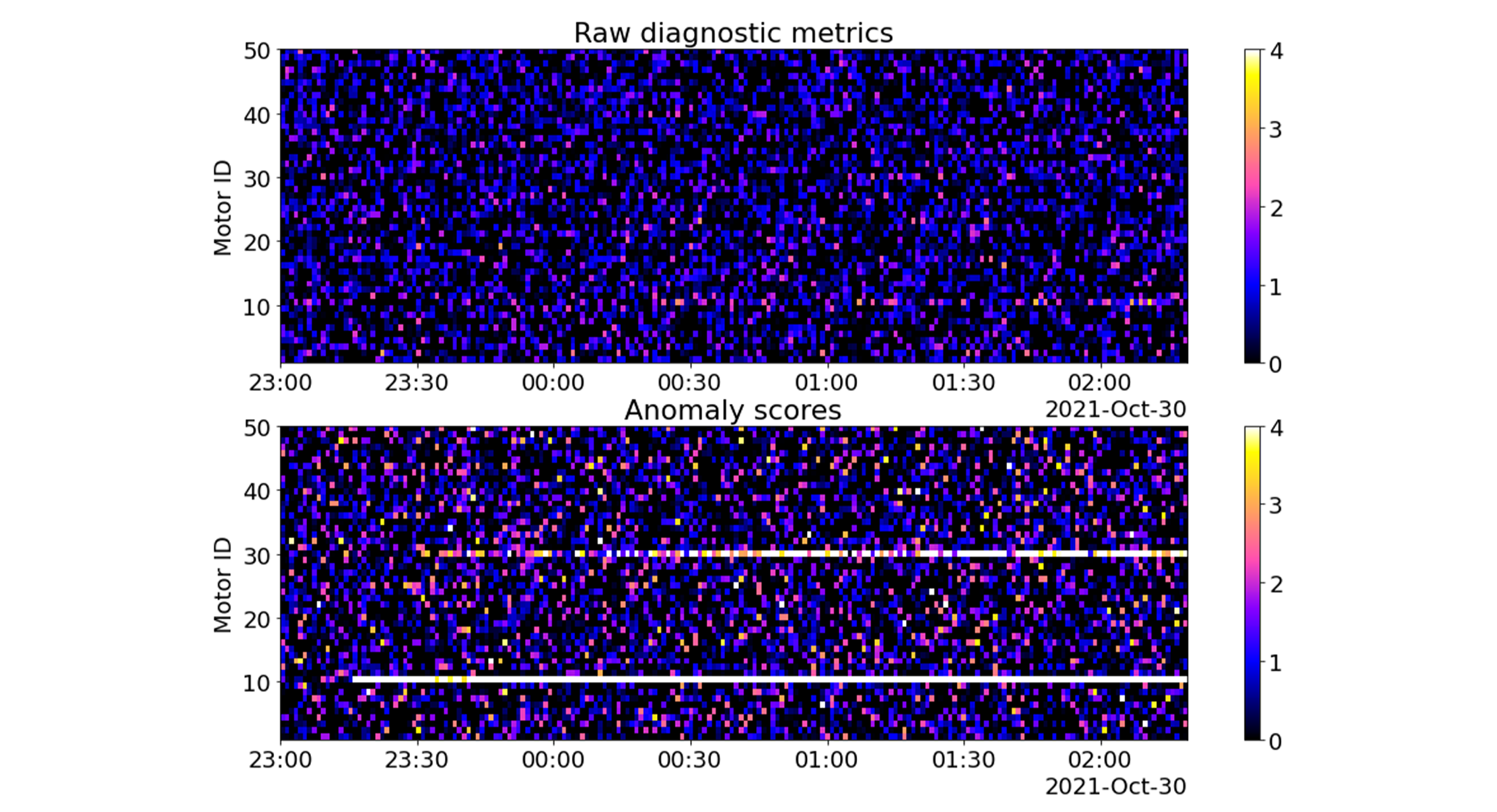
Even a cursory look at the figure above shows much higher sensitivity of the anomaly scores (bottom plate) compared to the primary metrics (upper plate). The anomalies are almost invisible in the primary metrics chart, but light up in the anomaly scores chart.

The Vertex AI Tabular Regression service also provides 95% confidence intervals for the prediction, which can be very useful for the purposes of anomaly detection. The figure below shows the estimated confidence intervals for all 50 motors for one particular time step, overlaid with the observed values of the vibration. This figure corresponds to the end of the time interval depicted in the above charts, so the anomalies in the 10th and 30th motors are well-developed and fall outside of the confidence interval.

Assuming the 95% confidence interval, we should also expect about 5% of the normal observations to fall outside of the estimated ranges. In the above figure, this is the case for the non-anomalous motors 6 and 9.

Anomaly detection based on scores

The anomaly scores described in the previous section are sufficient for visualization purposes, however, automated anomaly detection requires the development of an additional module that converts the soft scores into binary decisions.

If we have only one motor, the problem is rather simple. We can start with setting the target probability of false alarms and then compute the detection threshold to achieve this target. For example, the false alarm probability of $0.001$ can be achieved by choosing the $(1-0.001)$-th quantile of the score distribution as the threshold. It is also important to bear in mind that there is always a tradeoff between the false positive and false negative rates that needs to be settled based on the business and operational considerations.

The situation is more complex when we have many primary diagnostic metrics. In our running example with motors, we might be looking to assess the entire installation with 50 motors as a single system. This requires the development of some aggregation procedure which takes into account the anomaly scores for all motors simultaneously, and makes a decision about the overall health of the system.

One of the most straightforward solutions is to make binary decisions for each motor independently and then aggregate them using the OR operation: if at least one of the 50 motors is in an anomalous state, then the whole system is in an anomalous state too; otherwise the whole system is healthy. The disadvantage of this approach is that the optimization of the individual detection thresholds, with a goal to achieve a specific false positive rate for the entire system, can be intractable when the diagnostic metrics (motors in our case) are statistically dependent. This problem is known as multiple hypothesis testing.

The alternative approach is to aggregate the anomaly scores and then make the final binary decision using the thresholding procedure described above. As long as the individual anomaly scores $s_{i}$ have approximately equal variability for the healthy state, a simple average is a good choice for the aggregation function.

The anomaly detection process using score aggregation is illustrated in the charts below. First, we aggregate scores $s_{i}$ across all motors into a single statistic and compute the detection threshold to achieve the false positive rate of $0.01$ on the normal data:

Next, we evaluate the scores on the dataset with anomalies in the 10th and 30th motors, which we used in the previous section, and make the binary decisions based on the previously determined threshold:

Model deployment strategies

An IoT anomaly detection solution is more than just a model. An end-to-end solution must include integration with IoT sensors, data collection pipelines, model deployment and model monitoring capabilities. It is beyond the scope of this article to develop a complete solution architecture, but we outline the main model deployment strategies to give an idea of what the steps after the model development would look like:

• Cloud deployment. Many companies initially deploy anomaly detection models in the cloud. These models can be integrated into the production processes in two ways. One option is to score the ongoing metrics streams in a centralized way and send alerts back to the facilities. The alternative approach is to expose these models as services and invoke their APIs from edge devices to perform scoring.
• Edge deployment. Although the cloud deployment strategy can be used to perform near real-time scoring, the scoring latency might not be appropriate for manufacturing scenarios that require instant response on anomalies (e.g. defect detection on a conveyor belt). Such scenarios are often addressed by deploying the scoring model on edge servers. Being able to export your model to an edge device should be one of the considerations when evaluating different model architectures.
• Specifications for black-box suppliers. Many manufacturing companies work with suppliers that provide limited access to their production facilities and equipment. The two strategies described above might not be feasible for such suppliers, and manufacturers have to develop various workarounds. For example, suppliers can be provided with threshold-based specifications instead of model artifacts or APIs.

Advanced scenarios

In this blog post, we discussed the main approaches to anomaly detection and developed a basic prototype that demonstrates how the problem can be solved using off-the-shelf ML components. In practice, system health monitoring solutions often include a broader range of capabilities and leverage advanced modeling techniques. Here are several typical examples:

• Metric summarization and visualization. The journey towards system health monitoring usually starts with metric summarization and visualization. In complex environments, meaningful metric visualization can be a challenging problem that requires denoising and dimensionality reduction techniques.
• Large number of sensors. Some manufacturing environments deal with a very large number of sensors and metrics (e.g. 5000 metrics per machine). It can be challenging to detect anomalies and properly assess the impact of individual anomalies on the stability of the entire system with such high-dimensional signals. We discuss this problem in another blog post dedicated to anomaly detection in high-dimensional IoT data.
• Explainability. In practice, it is rarely enough to provide only basic anomaly detection functionality. In order to troubleshoot anomalies, operations teams need to be provided with insightful root cause analysis information and related anomalous samples need to be grouped together to simplify the investigation and prevent alert storms. These capabilities can be implemented using specialized methods such as group anomaly detection.
• Contextual anomalies. We already discussed that understanding the semantics of anomalies and external factors is critically important for meaningful anomaly detection. In some environments, we also need to account for the context in which the anomaly is happening. For example, metrics can be collected from different models of equipment and different operation modes can be used on weekdays and weekends. The context may or may not be explicitly observed. Specialized contextual anomaly detection algorithms can be used in such scenarios [3].
• Prescriptive guidance. In complex manufacturing environments, anomaly detection and troubleshooting is only a part of intelligence that can be provided to plant managers. Companies often perform side-by-side comparison of multiple locations and other types of analyses to provide plant managers with prescriptive guidance on possible improvements and prevent future failures.

Conclusions

The modeling methodology and reference pipeline developed in this article is based on multiple real-world projects implemented by Grid Dynamics. Although anomaly detection is usually considered as a separate class of ML problems, and there are multiple specialized algorithms for it, we demonstrated that many practical scenarios can be solved using generic components such as AutoML Forecasting, Regression, and Classification services provided by Vertex AI. Readers who are looking for a more comprehensive treatment of the anomaly detection theory are advised to consult the books and surveys dedicated to this topic such as [4].

References

1. Sipple J., Interpretable, Multidimensional, Multimodal Anomaly Detection with Negative Sampling for Detection of Device Failure, 2020
2. https://cloud.google.com/blog/products/data-analytics/bigquery-ml-unsupervised-anomaly-detection
3. Hayes, M.A., Capretz, M.A. Contextual anomaly detection framework for big sensor data, 2015
4. Aggarwal C., Outlier Analysis, 2017