Building a Next Best Action model using reinforcement learning

Modern customer analytics and personalization systems use a wide variety of methods that help to reveal and quantify customer preferences and intent, making marketing messages, ads, offers, and recommendations more relevant and engaging. However, most of these methods are designed to optimize only one immediate interaction with a customer and use objective functions defined through metrics like a click-through rate (CTR) or conversion rate (CR). This approach may or may not be a good approximation of real customer journeys that generally consist of multiple related interactions that can be jointly optimized with longer-term objectives in mind. This problem can be particularly important in industries like retail banking and telecom where customer relationships evolve over long periods of time.

In this tutorial, we discuss how traditional targeting and personalization models such as look-alike and collaborative filtering can be combined with reinforcement learning to optimize multi-step marketing action policies (aka Next Best Action policies). We use methods that were originally developed and tested by Adobe and Alibaba, and they proved to be effective in a number of practical use cases. ^[1][2] For this tutorial, we chose to use a simple testbed environment with synthetic data to explain the model design and implementation more cleanly; we will present a practical case study in another blog post.

Basics of customer intent analysis

To put the problem of multi-step optimization of marketing actions into context, let's start with one of the most basic and widely used targeting methods – look-alike modeling. The idea of look-alike modeling is to personalize ads or offers based on the similarity of a given customer to other customers who have exhibited certain desirable or undesirable properties in the past. Consider the classic example of a subscription service provider that seeks to prevent customer churn by distributing a retention offer. Assuming that each offer is associated with some costs to the provider, we should only target a limited subset of customers with a high risk of churn. We can approach this problem by collecting a number of historical customer profiles that can include both demographic and behavioral features, attributing those features with the observed outcomes (churn or no churn), training a classification model based on these samples and then using this next best offer machine learning model to score the level of churn risk for any given customer to determine whether the offer should be issued or not:

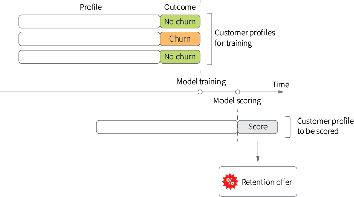
This approach provides significant flexibility, in the sense that models can be built for a wide variety of business objectives depending on how the outcome label is defined: it can be a propensity to try a new product, propensity to upsell, proximity to a brand or channel and many others. It also works well in a variety of environments, including online advertising and retail promotions.

The solution described above can be extended in a number of ways. One of the apparent limitations of basic look-alike modeling is that models for different outcomes and objectives are built separately, and the useful information about similarities between offerings is ignored. This issue becomes critical in environments with a large number of offerings, such as recommendation systems. Typically, the problem is circumvented by incorporating user features, offering features and a larger user-offering interaction matrix into the model so that interaction patterns can be generalized across the offerings; it is done in many collaborative filtering algorithms, including ones that are based on matrix factorization, factorization machines and deep learning methods:

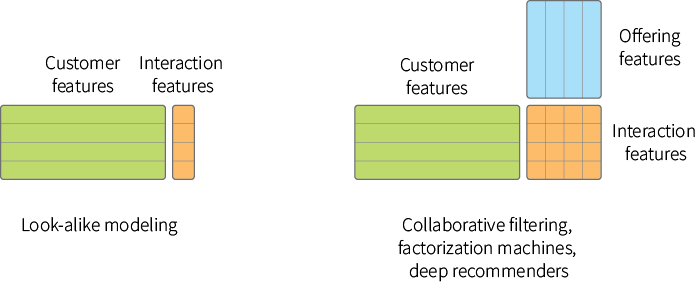
Next best action predictive models help to predict customer intent more accurately by incorporating a wider range of data, including features extracted from texts and images, but this is not particularly useful for optimizing multi-step action strategies.

The problem of strategic optimization can be partly addressed by a more careful design of the target variable, and this group of techniques represents the second important extension of basic look-alike modeling. The target variable is often designed to quantify the probability of some immediate event like a click, purchase, or subscription cancellation, but it can also incorporate more strategic considerations. For example, it is common to combine look-alike modeling with lifetime value (LTV) models to quantify not only the probability of the event, but also its long term economic impact (e.g. what will be the total return from a customer retained from churn or what will be a 3-month spending uplift after a special offer):

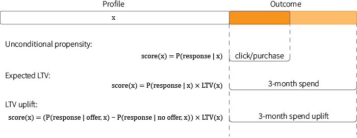
These techniques help put the modeling process into a strategic context, but do not really provide a framework for optimizing a long-term marketing communications strategy. So our next step will be to develop a more suitable framework, specifically for this problem.

Customer journey as a markov decision process

The problem of strategic (multi-step) optimization of marketing communications stems from the stateful nature of customer relationships and dependencies between marketing actions. For example, one can view retail offer targeting as a single-step process where a customer can either be converted or completely lost (and train a model that maximizes the probability of conversion):

However, the real retail environment is more complex and customers can interact with a retailer multiple times before a conversion occurs, and the customer makes related purchases. Consider the following scenario of a promotion campaign:

1. Inform customers about product features and additional packages through an ad.
2. Announce a special offer that incentivizes customers to buy a product by providing a discount on the second purchase ("Buy X, and save on your next shopping trip").
3. After the first purchase, customers are incentivized to make a second purchase to redeem the special offer.

It is clear that all actions in the above strategy are related, and their order is important. For instance, the initial ad alone may not increase conversions, but it can boost the efficiency of the downstream offers. It can also be the case that the ad is most efficient if issued not in the beginning of the conversation, but between the announcement and the offer, and so on.

The complex structure of a customer journey plays an even more important role in industries like banking and telecom. In retail banking, a customer can start with a basic product like a checking account, then open up a credit card account, then apply for brokerage services or a mortgage; customer maturity grows over time, and offerings need to be sequenced properly to account for this.

The above use cases can be naturally represented as Markov Decision Processes (MDP), where a customer can potentially be in several different states and move from one state to another over time under the influence of marketing actions. In each state, the marketer has to choose an action (or non-action) to execute, and each transition between states corresponds to some reward (e.g. number of purchases), so that all rewards along the customer trajectory sum up to a total return that corresponds to customer LTV or campaign ROI:

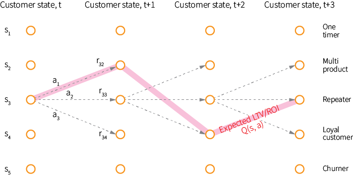
Although one can use a hand-crafted set of states with clear semantic meaning, we will assume the state is represented simply by a customer feature vector, so that the total number of states can be large or infinite in the case of real-valued features. Note that the state at any point of time can include records of all previous actions taken with regard to this customer.

In the MDP framework, our goal is to find an optimal policy $\pi$ that maps each state to the probabilities of selecting each possible action, so that $\pi(a\ |\ s)$ is the probability of taking action $a$, given that a customer is currently in state $s$. The optimality of the policy can be quantified using the expected return under this policy – the expected sum of rewards $r$ earned at each transition.

A naive solution for this problem is to build multiple look-alike models for different actions and different designs of the training labels similar to the following:

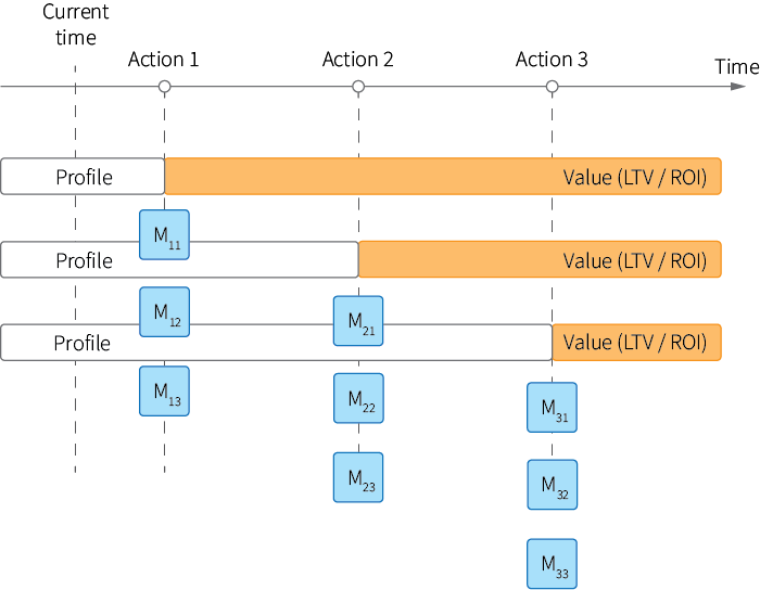
In this approach, we first build a set of models $M_{11}, M_{12}, \ldots$ for each action allowed in the initial state, using profiles of customers who received this action in the past and with the target label defined over a long period of time. This label is a direct estimate of the expected return. We then build a second set of models $M_{21}, M_{22}, \ldots$ using customer profiles with features that indicate which action was taken first, and so on. In other words, we optimize actions sequentially using the fact that "good" customer trajectories start with "good" initial actions for given customer characteristics.

However, this naive approach is computationally inefficient, requires building multiple models, and cannot be easily adopted for online learning. We can expect to achieve higher efficiency and flexibility using reinforcement learning algorithms that solve a generic MDP problem.

Solving MDP using Fitted Q Iteration

In order to apply generic reinforcement learning algorithms, let us introduce a few additional concepts that build on the MDP framework and the notions of state, action, reward and policy that we previously defined.

Assuming that we have some policy $\pi$, let us introduce the action-value function $Q_{\pi}$ that quantifies the value of taking action $a$ in state $s$, as the expected return starting from $s$, taking action $a$ and following policy $\pi$ after that:

$$
Q_{\pi}(s, a) = \mathbb{E}_ \pi \left[ \sum_{t \ >\ t_s} r_{t} \ |\ s, a \right]
$$

The action-value function can be estimated based on the feedback data (customer trajectories in our case) collected under policy $\pi$. At the same time, the policy itself can be improved based on the estimated action-value function. The most basic way to do this is to simply take the action with the maximum expected value at each state (and, consequently, the probabilities of all other actions in this state will be zero):

$$
\pi(s) = \underset{a}{\text{argmax}}\ Q_{\pi}(s, a)
$$

Thus, the process of learning the optimal policy can be iterative: we can start with some baseline policy, collect the feedback data under it, learn the action-value function from this data, update the policy and repeat the cycle again.

Next, we need an algorithm for the action-value function estimation. The theory of reinforcement learning offers a wide range of such algorithms that are designed for different assumptions about the MDP environment. In the most basic case, one can assume a fully known, deterministic and computationally tractable environment, so that all states, actions, and rewards are known. In this case, the action-value function can be straightforwardly estimated using classic dynamic programming: we simply compute the total returns for different states as the sums of rewards on the paths in the MDP trellis that originate in these states. It is not even a machine learning problem, but a purely computational problem. However, real environments often impose additional challenges that make this basic approach infeasible and require the development of more advanced and specialized algorithms:

• Generalization. The number of states or transitions can be very large or infinite. In this case, the training data (trajectories) we have, might not cover all states and we need to generalize our observations using next best action machine learning techniques.
• Online learning and exploitation. We might have little or no historical data, and learn reward values and states online by trial and error. It leads to the exploration-exploitation problem: the more time we spend on exploring the environment and learning what works and what does not, the less time we earn high rewards by making optimal actions according to the best policy we learned.
• Off-policy evaluation and learning. As we previously mentioned, policy learning is generally an incremental process where policy testing and action-value function re-estimation repeats iteratively. In many environments, including marketing, we have a limited ability to test arbitrary policies because they can lead to inappropriate customer experiences or other issues. This means that we might need to learn and evaluate policies based on the feedback data generated under other policies.

All these challenges are relevant to our use case: the customer state is defined by the vector of real-valued features making the total number of states unlimited, and we generally need to test and adjust our policy on real customers even if we have historical data to start with.

The first problem of generalization across the states is addressed by a number of different reinforcement learning algorithms. In fact, we have already seen how this generalization can be done using look-alike modeling when we discussed our naive algorithm for multi-step optimization. The more efficient and generic solution for this problem is Fitted Q Iteration (FQI) algorithm. ^[3][4]

The idea of the FQI algorithm is to reduce the problem of learning the action-value function to a supervised learning problem. This is done with the iterative application of some supervised learning algorithm; we first train the model to predict the immediate reward based on state and action features, then train the second model to predict the return for two time steps ahead, and so on.

More specifically, let us assume that we have a number of trajectories collected under some baseline policy, and we cut these trajectories into a set of individual transitions, each of which is a tuple of the initial state, action, reward and new state:
$$
T = \{ (s, a, r, s’) \}
$$

The FQI algorithm then can be described as follows:

State $s_i$ and action $a_i$ are assumed to be vectors representing state and action features, reward $r$ is assumed to be a scalar value, and $0 \le \gamma \le 1$ is a discount rate that can be used to control the tradeoff between immediate and long-term rewards.

The algorithm is quite straightforward: we start with a short-sight approximation of the action-value function, and then adjust the training label at each iteration to backpropagate the reward. The FQI algorithm can use any supervised learning algorithm to approximate the $Q$ function; the typical choices are random forest and neural networks (Neural FQI).

In the next sections, we build a prototype of the Next Best Action machine learning model using this approach. We will address the online and off-policy learning aspects of the problem in the later sections as well.

Setting up a testbed environment

We start building the Next Best Action model by setting up a simple testbed environment. First, let us assume a customer can do one of the following actions at any time step: take no action, visit a website or store without a purchase, or make a purchase. Let us also assume that a seller can provide a customer with one of three offers at any point of time or decide not to provide any offer. For the sake of illustration, we assume the semantic meaning of these offers are advertisement, small discount and large discount, respectively. For the sake of completeness, we also assume that customers have demographic and behavioral features. Without loss of generality, we use just one feature that can be either zero or one depending on the age group:

events = [
    0, # no action
    1, # visit
    2  # purchase
]
offers = [
    1, # advertisement
    2, # small discount
    3  # large discount
]
demographic = [
    0, # young customers
    1  # old customers 
]

Next, let's assume that we have some historical data at our disposal to learn the offer targeting policy. We create a customer profile generator that simulates three historical offer campaigns. For each customer, this generator iterates over 100 time steps, and issues three offers at randomized points of time. We initially use a random targeting policy, so that all offers have the same probability regardless of customer features. Customer behavior (i.e. event probabilities) changes over time as a function of previously received offers, and also depending upon demographic features:

k = 100            # number of time steps
m = 3              # number of offers (campaigns)
n = 1000           # number of customers

def generate_profiles(n, k, m):
    p_offers = [1 / m] * m                                      # offer probabilities 
    t_offers = np.linspace(0, k, m + 2).tolist()[1 : -1]        # offer campaign times
    t_offer_jit = 5                                             # offer time jitter, std dev 
    
    P = np.zeros((n, k))                                        # matrix of events
    F = np.zeros((n, k))                                        # offer history
    D = np.zeros((n, 1))                                        # demographic features

    for u in range(0, n):
        D[u, 0] = np.random.binomial(1, 0.5)                    # demographic features
    
        # determine m time points to issue offers for customer u
        offer_times_u = np.rint(t_offer_jit * np.random.randn(len(t_offers)) + t_offers)
        
        for t in range(0, k):                                   # simulate a trajectory
            if t in offer_times_u:
                F[u, t] = multinomial_int(p_offers) + 1         # issue an offer at time t 
   
            event = multinomial_int(get_event_pr(D[u], F[u]))   # generate an event at time t
            P[u, t] = event
        
    return P, F, D

This generator produces three matrices:

• $P$ — $n \times k$ matrix of customer events
• $F$ — $n \times k$ matrix of offers issued to customers
• $D$ — $n \times 1$ matrix of customer demographic features

The most important part of the simulator is a mapper of customer profiles to the vector of event probabilities. We define this mapper in such a way that the probability of a purchase is boosted if and only if the offer #1 (advertisement) is followed by the offer #3 (large discount):

def get_event_pr(d, f):
    f_ids = offer_seq(f)     # sequence of offer IDs received by the customer
    f_ids = np.concatenate((offer_seq(f), np.zeros(3 - len(f_ids))))
    
    if((f_ids[0] == 1 and f_ids[1] == 3) or 
       (f_ids[1] == 1 and f_ids[2] == 3) or 
       (f_ids[0] == 1 and f_ids[2] == 3)): 
            p_events = [0.70, 0.08, 0.22]     # higher probability of purchase
    else:
        p_events = [0.90, 0.08, 0.02]         # default behavior
        
    if(np.random.binomial(1, 0.1) > 0):       # add some noise
        p_events = [0.70, 0.08, 0.22]
    
    return p_events

Our goal will be to build a model that can recognize this type of dependency. For the sake of simplicity, we ignore demographic features when choosing the event probabilities, but the design of the model we develop is fully capable of learning these dependencies as well.

Next, we generate and visualize the training and test data sets:

P, F, D = generate_profiles(n, k, m)          # training set
Pt, Ft, Dt = generate_profiles(n, k, m)       # test set

visualize_profiles(P)
visualize_profiles(F)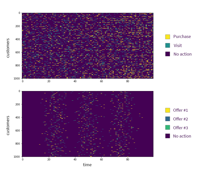

We can see in the top chart that the frequency of purchases increases over time (the density of the yellow dashes increases from left to right) because some customers get the right sequence of offers that triggers an increase in the purchase probability.

Estimating the action-value function

Our next step is to learn the offer targeting policy using the FQI algorithm we introduced earlier. FQI works with individual transitions, so we need to cut the trajectories we previously generated into pieces as follows:

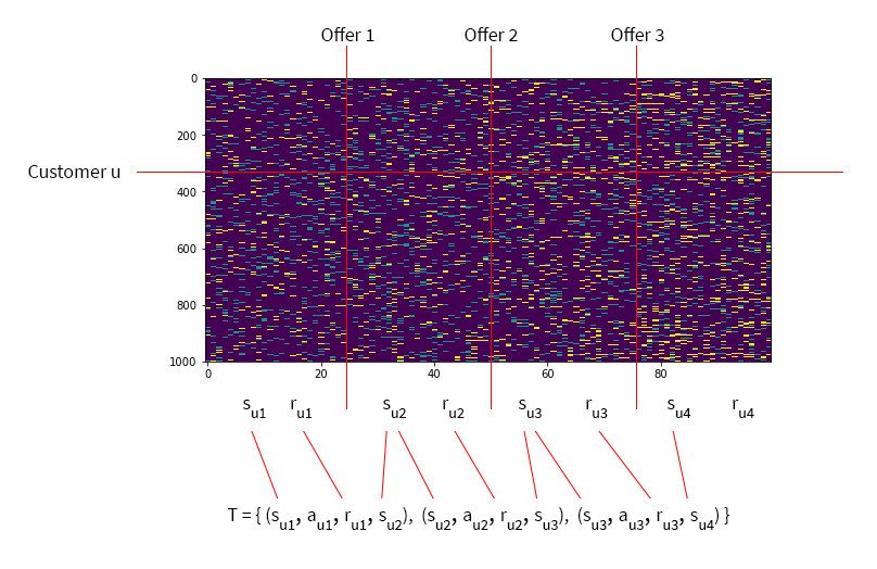
This way, each customer trajectory produces several transition tuples, and all tuples are merged into one training set. We choose to use the number of purchases in each transition as the reward metric, and represent each state as a vector of the following features: a demographic feature, the total number of visits from the beginning of the trajectory and time steps at which offers of each type were issued:

# p, f, d - rows of matrices P, F, and D that correspond to a given customer
# t_start, t_end - time interval 
def state_features(p, f, d, t_start, t_end):
    p_frame = p[0 : t_end]
    f_frame = f[0 : t_end]
    return np.array([
        d[0],                  # demographic features
        count(p_frame, 1),     # visits
        index(f_frame, 1, k),  # first time offer #1 was issued
        index(f_frame, 2, k),  # first time offer #2 was issued
        index(f_frame, 3, k)   # first time offer #3 was issued
    ])

def frame_reward(p, t_start, t_end):
    return count(p[t_start : t_end], 2)   # number of purchases in the time frame

The following snippet contains the full code for cutting trajectories into transitions.

Click to expand the code sample (27 lines)

def prepare_trajectories(P, F, D):
    T = []
    for u in range(0, n):
        offer_times = find_offer_times(F[u]).tolist()
        ranges = offer_time_ranges(offer_times)
        
        T_u = []
        for r in range(0, len(ranges)):
            (t_start, t_end) = ranges[r]
            state = state_features(P[u], F[u], D[u], 0, t_start)
            reward = frame_reward(P[u], t_start, t_end)
            state_new = state_features(P[u], F[u], D[u], t_start, min(t_end + 1, k))
            
            if(t_end in offer_times): 
                action = F[u, t_end]
            else:
                action = 1 
                
            T_u.append([state, action, reward, state_new])
            
        T.append(T_u) 
        
    return np.array(T)

def offer_time_ranges(times):
    rng = [-1] + times + [k]
    return list(zip(map(lambda x: x + 1, rng), rng[1:]))

We use it to prepare both training and test sets of transitions:

T = prepare_trajectories(P, F, D)
Tt = prepare_trajectories(Pt, Ft, Dt)

Once the data is ready, we can apply the FQI algorithm to learn the action-value function. We use the random forest algorithm from scikit-learn as a subroutine for $Q$ function estimation:

def Q_0(sa):
    return [1]

Q = Q_0
iterations = 6
for i in range(iterations):                 # FQI iterations
    X = []
    Y = []
    for sample in T.reshape((n * (m + 1), m + 1)):
        x = np.append(sample[0], sample[1]) # feature vector consists of state-action pairs
    
        a_best, v_best = best_action(Q, sample[3], offers)
        y = sample[2] + v_best              # reward + value
    
        X.append(x)
        Y.append(y)
    
    regr = RandomForestRegressor(max_depth=4, random_state=0, n_estimators=10)
    regr.fit(X, np.ravel(Y))    
    Q = regr.predict

# find the optimal action under a greedy policy and corresponding state value
def best_action(Q, state, actions):
    v_best = 0
    a_best = 0
    for a in actions:
        v = Q([np.append(state, a)])[0]
        if(v > v_best):
            v_best = v
            a_best = a
            
    return a_best, v_best

Next, we can use the action-value function to make Next Best Action recommendations for the test set. It is insightful to visualize these recommended actions and corresponding action-value function estimates:

Click to expand the code sample (21 lines)

# use the test set to evaluate the policy
states = Tt[:, :, 0].flatten().tolist()

values = []
best_actions = []
for s in states:
    a_best, v_best = best_action(Q, s, offers)
    values.append(v_best)
    best_actions.append(a_best)

s_tsne = TSNE().fit_transform(states)

# value function for each state
plt.scatter(s_tsne[:, 0], s_tsne[:, 1], c = values)
plt.colorbar()
plt.show()

# recommended next best actions for each state
plt.scatter(s_tsne[:, 0], s_tsne[:, 1], c = best_actions)
plt.colorbar()
plt.show()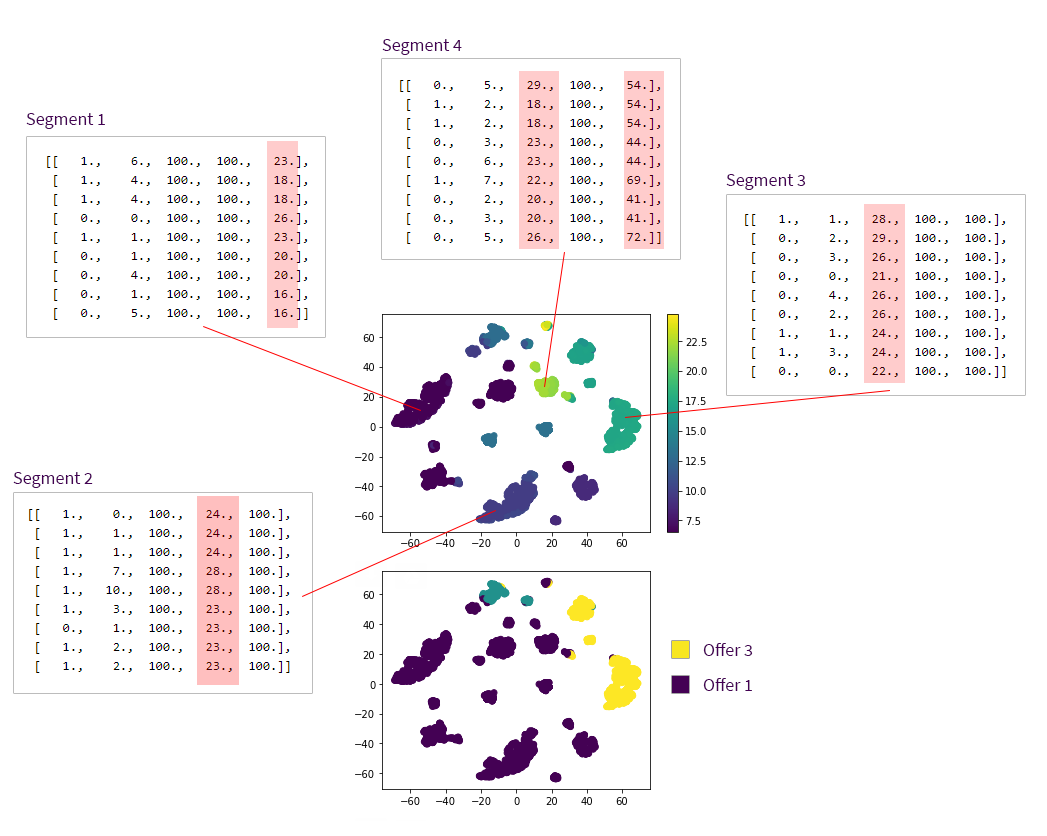

The top scatter plot shows the value of the best action for each customer state, and the bottom plot shows the recommended next best action for each state. The two plots are identical except for the color coding. We can see several clusters of customer states (segments) with different expected values and recommended actions. As we previously described, each state in our model is represented by a vector of five features (demographic, number of visits and issue times for each of three offers), so it is useful to pull a few samples from each of these segments and examine them:

• Segment 1. These are the customers who got offer #3 in the beginning of the trajectory. Our generative model boosts the purchase probability only if offer #1 precedes offer #3, so these customers are lost causes with minimum value.
• Segment 2. These customers got offer #2 first. The model rightly recommends to give them offer #1 next, but the predicted value for this segment is relatively low because the remaining time until the end of the trajectory is limited.
• Segment 3. These customers got offer #1 first, and the model recommends to give them offer #3 next. The expected value is relatively high because these customers are on the right track.
• Segment 4. These customers already got offer #1 followed by offer #3, and it boosted their purchase rates. They have the highest expected values. The system recommends providing them offer #1 as a default action, but the recommended action does not make any difference because the right offer combination has already been unlocked by that time.
  
  

Evaluating the Next Best Action policy

The FQI algorithm provides a way to estimate the action-value function based on historical data obtained under some previous policy. We need to convert the action-value function into the Next Best Action policy, which can be done in several different ways. We have already seen that it can be done by taking the action with the highest expected value and zeroing the probabilities of taking any other action allowed in a given state. This approach produces a greedy policy that focuses exclusively on earning rewards according to the currently known policy and does not explore alternative (non-optimal) actions in order to improve the policy.

Since the learning process is typically interactive or even online, and the data obtained under the first policy produced by FQI is then used to learn the next policy, it is common to use an epsilon-greedy policy that randomly explores non-optimal actions with some small probability defined by the hyperparameter $\epsilon$:

$$
\pi_{\epsilon} (s, a) =
\begin{cases}
1-\epsilon, & \text{if } a = \underset{a}{\text{argmax}}\ Q_{\pi}(s, a) \\
\epsilon/(m-1), & \text{otherwise}
\end{cases}
$$

where $m$ is the total number of actions allowed in the state. This gives more bandwidth for exploration and policy improvement. In dynamic online environments, the policy can be updated many times, and parameter $\epsilon$ can also be dynamically adjusted depending on the volatility of observed feedback. ^[2:1]

The second problem that needs to be addressed is estimating the expected return under the optimized policy before this policy is applied in production. It can be needed to ensure that the new policy meets service quality and performance standards, and may also be required to tune parameters of the policy such as the value of $\epsilon$ in the epsilon-greedy policy.

This policy evaluation can be done using historical trajectories generated using the previous policy, and rescaling the returns proportionally to the differences between the policies. Assuming that we have a trajectory generated using some baseline policy $\pi_0$ that consists of a series of states $s_t$ and actions $a_t$, we can estimate the return of a new policy $\pi$ as follows:

$$
\widehat{R}(\pi) = R(\pi_0) \prod_t \frac{\pi(s_t, a_t)}{\pi_0(s_t, a_t)}
$$
where $R(\pi_0)$ is the observed return of the trajectory. Averaging this estimate over a set of trajectories, we can evaluate the overall expected performance of a policy. This method is called importance sampling estimation.

The implementation of the policy evaluation using importance sampling is straightforward:

def evaluate_policy_return(T, behavioral_policy, target_policy):
    returns = []
    for trajectory in T:                                                   
        importance_weight = 1
        trajectory_return = 0
        for transition in trajectory:            
            state, action, reward  = transition[0 : 3]
            action_prob_b = behavioral_policy(state, action)
            action_prob_t = target_policy(state, action)
            
            importance_weight *= (action_prob_t / action_prob_b) 
            trajectory_return += reward
            
        returns.append(trajectory_return * importance_weight)
        
    return np.mean(returns)

We use this evaluation procedure to quantify how the expected performance of an epsilon-greedy policy depends on the $\epsilon$ parameter:

policy_values = []
eps = np.linspace(0, 2/3, num = 10)
for e in eps:
    policy = make_epsilon_greedy_policy(e)
    policy_values.append( evaluate_policy_return(T, behavioral_policy, policy) )

plt.plot(eps, policy_values)
plt.show()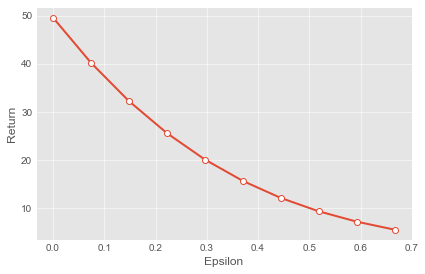

Importance sampling and other off-policy evaluation methods provide a way to do safety checks and modifications before a new policy is deployed in production.

Conclusions

Reinforcement learning provides a convenient framework for building Next Best Action models that generally need to combine predictive analytics, combinatorial optimization and active exploration of a dynamic environment. The ability to combine these elements in different ways is one of key advantages of the reinforcement learning framework. For instance, a basic offering optimization problem that requires only experimentation can be solved using multi-armed bandit algorithms. Then, the information about customers and offerings can be incorporated using contextual bandits, and then more strategic decisions can be made using generic reinforcement learning algorithms in a way described in this article. Finally, even more complex models can be created using deep reinforcement learning methods such as DQN. ^{[2:2] [5]}

The second advantage of the reinforcement learning approach is the flexibility of modeling. Similar to Monte Carlo simulations, it allows the incorporation of additional requirements, such as budgetary constraints, operational costs and business restrictions, by redefining reward functions or action sets. This provides more flexibility as compared to the manual casting of the optimization problem to some standard form, like linear or integer programming.

The same approach can be applied in many other areas of enterprise operations, including marketing, pricing, and logistics. For example, we discussed how multi-armed bandits can be used for dynamic price optimization in a previous blog post, and we can take this approach further using the MDP framework.

The complete implementation of the testbed environment described in this article is available on github. We used just plain python and scikit-learn to implement our toy model, but it is highly advisable to use reinforcement learning frameworks like OpenAI Gym for real production implementations to reliably handle all aspects and edge cases of modeling and optimization.

References

---

1. G. Theocharous, P. Thomas, and M. Ghavamzadeh, Personalized Ad Recommendation Systems for Life-Time Value Optimization with Guarantees, 2015 ↩︎

2. D. Wu, X. Chen, X. Yang, H. Wang, Q. Tan, X. Zhang, J. Xu, and K. Gai, Budget Constrained Bidding by Model-free Reinforcement Learning in Display Advertising, 2018 ↩︎ ↩︎ ↩︎

3. D. Ernst, L. Wehenkel, and P. Geurts, Tree-based batch mode reinforcement learning. Journal of Machine Learning Research, 2005 ↩︎

4. M. Riedmiller, Neural Fitted Q Iteration - First Experiences with a Data Efficient Neural Reinforcement Learning Method, 2005 ↩︎

5. V. Mnih et al, Human-level Control Through Deep Reinforcement Learning, 2015 ↩︎