Building a Workforce Schedule Optimization solution

When it comes to human capital, many organizations face a lingering dilemma concerning workforce management. There are two extremes: overstaffing and understaffing. Overstaffing leads to underuse of existing employees and causes labor costs to increase. Understaffing, on the other hand, cripples the company’s ability to maintain the desired level of customer service and has a negative impact on staff morale due to excessive overtime.

To find the best solution to this dilemma, organizations have to strike a balance between staffing costs and service levels. But first of all they need to ask themselves:

1. What demand is expected in future?
2. What is the minimum number of employees needed to meet this demand?

These questions reveal that the problem is actually twofold. The first component is demand forecasting, which is the central point in personnel planning.The second component refers to schedule optimization aimed at minimizing costs despite various constraints (i.e. business rules, service level requirements).

In this article we will describe a general solution architecture that enables you to tackle these issues in a timely manner. It was developed by Grid Dynamics and has already been utilized in multiple use cases proving its efficiency.

Workforce scheduling solution architecture

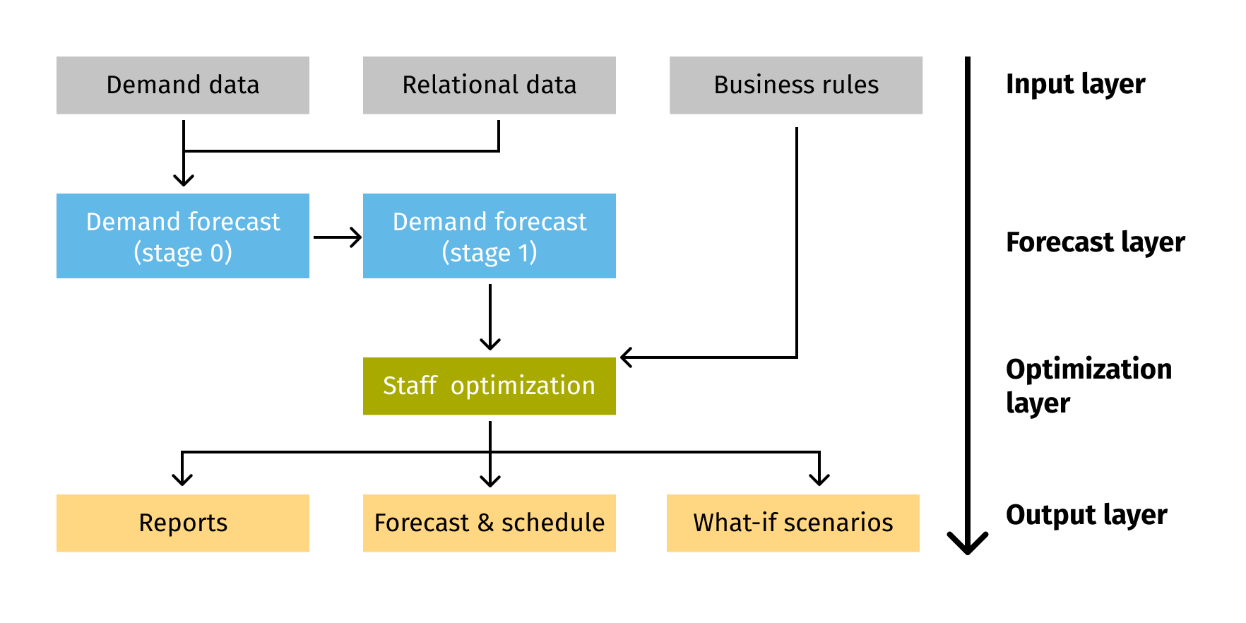
Our workforce schedule optimization solution has four layers (see the related chart):

1. Input layer is concerned with data preprocessing and feature selection. It utilizes three input datasets – demand data, relational data, and business rules. The first two are used in forecasting, while the latter aids staff optimization.
2. Forecast layer features a stacked model that can improve forecasting accuracy by creating a strong learner from weak learners.
3. Staff Optimization model is created using the outputs from the forecasting model as well as business rules and service level constraints.
4. Output layer offers forecasting and optimization outputs. With this modeling structure, it is possible to create different reports (e.g. planning and staffing) and run what-if scenarios.

You can take your parameter settings as a starting point for further fine-tuning, and then adjust this model architecture to various practical use cases. If you apply it for demand forecasting, it is possible to change input features in stage 0 and select different model types for stacking in stage 1. In the optimization model, our solution has the flexibility to add/remove business requirements to justify future needs and objectives. In addition, it allows for assessing the cost of each constraint and its impact on service level KPIs.

Work demand forecasting methodology

When choosing a forecasting model, business owners typically compare the performance of various methods (e.g. ARIMA and FB Prophet) and choose the best one based on the validation testing. However, this approach doesn’t allow the incorporation of the advantages of different algorithms into a single solution. For example, ARIMA captures the causal relationship between past and future but it fails to recognize trends and seasonality like FB Prophet does.

If you want to enjoy all the benefits workforce management software has to offer it is better to use model ensemble methods. There are three major methods of model ensembling: bagging, boosting and stacking.

• Bagging is the simplest ensemble technique in which several models train independently and the final prediction is the result of forecasts aggregation.

• Boosting is a widely-used model known for its great performance. It enables sequential training of similar models that can improve the prediction of weak learners in each step (such as XGBoost, LightGBM, CatBoost, etc.).

• Stacking is a common technique that utilizes the combination of different models. Here, several models are trained independently and their predictions are used as input for the Meta model.

Each of these methods has its pros and cons (see the table below).

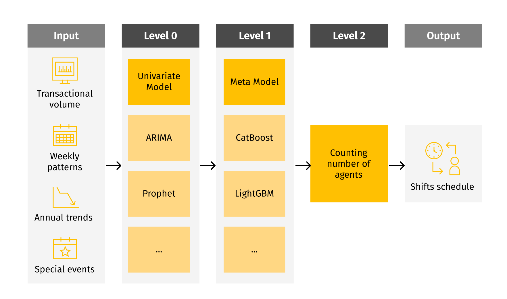
Considering the pros and cons of different ensembling techniques, we find that using stacking models with boosting as the meta model is the best approach for schedule optimization. The scheme below shows how it works:

Workforce optimization solution methodology Optimization solutions enable companies to make the best decision for the business, balancing several factors. In case of workforce scheduling optimization, the goal is to find the minimum number of working agents covering forecasted demand.

There are two main optimization methods: rule-based and ML-based. Rule-based optimization is built on “if-then” rules set by business requirements. It requires a deep understanding of business problems and a close connection with business stakeholders. Solutions rely on the knowledge built into the optimization part and give the output based on the current state of the business environment.

The upside of rule-based optimization is transparency and clear reasons for output. If needed, outputs can be adjusted manually which is important for decision making. On the downside, the algorithm needs to be changed every time the rule changes, which adds complexity to solution maintenance.

The ML-based approach incorporates optimization within the model solution. The idea is to use asymmetric objective function during the model training with predefined coefficients of asymmetry. This helps to reduce maintenance efforts. However, the solution needs to run A/B tests to check the model quality and determine the right coefficients. In addition, it has low explanatory power (see Safety stock optimization for Ship-from-Store).

Both approaches have their pros and cons but the final choice should be made based on the business requirements.

In our case studies, we provided both ML-based optimization (Case Study 1), and rule-based (Case Study 2) optimization examples.

Case Study 1: Schedule optimization for a call center

Our client, a leading telecommunications company, wanted to optimize their operational schedule for their call center which provides engineering support to different network services. The main task was to predict the demand in each network and estimate how many engineers were needed per shift.

Grid Dynamics was engaged in the development of a cutting-edge AI model that would enable strategic resource and operational planning. Our team created a stacked model to improve operational forecasting. We also built an optimization model to minimize operation costs subject to business and operational constraints.

Forecasting

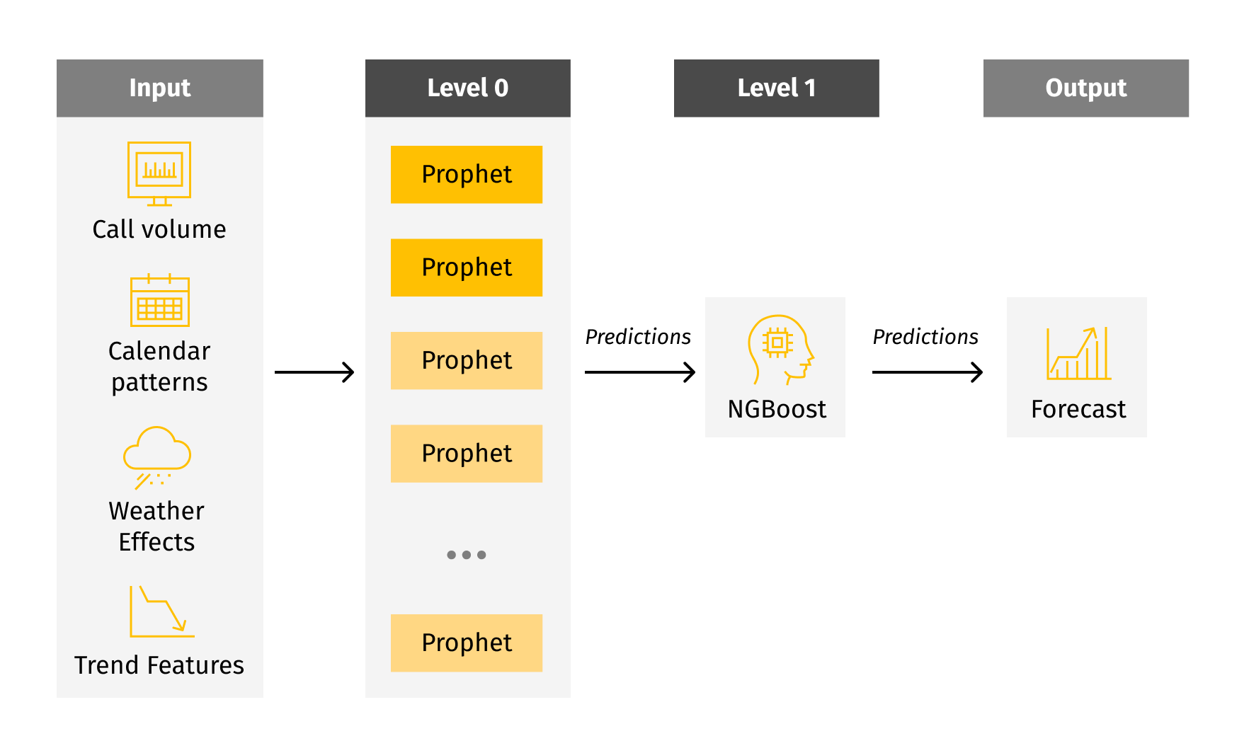
Prophet and ARIMA were used in level 0, while NGBoost was used in level 1. The solution takes inputs from four data categories – call volume (demand), calendar patterns (date), weather effects (weather-normalized assumptions for long-term predictions) and trend features. It offers flexibility to accommodate different machine learning models at each level (see the chart below).

ML-based optimization

The goal of the optimization model was to determine the minimum number of engineers required to meet demand and target service levels. Thus we have the following maximization function:

$$
\min \sum_{w \in W} \sum_{s \in S} c_s t_s x(w, s, t_s)
$$

Subject to:

• Forecast Demand and Service Level Targets (such as average handling time and call abandon rate). Supply should be greater than demand after accounting for unavailable time and available time buffer. E.g.
  $(1-b)*\sum x(w, s, t_s) \ge V_{dh} * \tau *(1-r)$
• Business Constraints (such as minimum staffing. E.g. $x(w,s,t_s) \ge m_s$)

Where

• $w$ is the day in the work schedule
• $s$ is the shift type
• $c_s$ is the shift cost
• $t_s$ is the shift length
• $x(w, s, t_s)$ is the number of engineers
• $V_{dh}$ is the demand volume
• $\tau$ is the average handling time
• $r$ is the call abandonment rate
• $b$ is the unavailable time buffer
• $m_s$ is the minimum staffing

In order to solve this optimization problem, we used the solver from Python’s PuLP library. PuLP is a linear programming modeler written in python.

Model output

The output of the model was an operational shift schedule. It helps the company with resource planning and to configure automatic scheduling. It also allows them to feed data on engineers’ availability into the model output and create a shift schedule at the individual level. This eliminates the need for dozens of scheduling spreadsheets scattered across different engineering teams and enables staff to update changes (e.g. vacation plans) in a matter of seconds.

Our model also helps the company to understand the cost impact from each business constraint. For example, to evaluate the impact of average wait time, we can set it to low/mid/high level and simulate the dynamics of costs. This sort of simulation helps organizations to make smart decisions on service level targets and presents possible ways to overcome business constraints.

Case study 2: Schedule optimization for offline stores

This use case aims to solve the problem of shifts scheduling in offline stores. Our client has agents working at brick-and-mortar facilities who provide assistance and services to customers. There are a number of transactions and the average time that employees spend on each transaction type and shift scheduling depends on the transactions’ number and length.

Grid Dynamics was engaged to deploy and maintain an AI solution that allowed for strategic resource planning and cost reduction. We created the model for transaction forecasting and schedule optimization.

Forecasting

We used a stacked model approach. There were two univariate models on level 0 – ARIMA and Prophet. On level 1 they were stacked with additional features into a LightGBM model.The feature preparation stage consisted of three steps:

1. Technical preparation was made, i.e. converting data types, filling missing values, etc.
2. Building features from raw data, i.e. correlations between parameters, different groupings, etc.
3. Adding analytical features, such as lags of transaction history, number of days before and after holidays, distance to competitor stores etc.

Historical time series trends were picked up by univariate models. In this case, LightGBM was chosen as the meta algorithm due to its accuracy. It takes into account not only historical trends of time series but also numerical and categorical features.

Prediction of transaction volume is made for a certain period of time (one week, one month or 60 days) which depends on business needs . The algorithm for each day was trained in an independent model with the same structure. The model quality was evaluated using the WMAPE metrics.

Rule-based optimization

At this stage, the number of agents in each shift was determined by the predicted number of transactions(see the formula below). The average transaction time was estimated based on historical data.

Number of agents in shift = (predicted number of transactions * average time on this transaction) / number of working hours

Model output

There are two model outputs. First, we got the number of transactions that were forecasted for a specified period. And secondly, we calculated the number of agents that were needed at work at the given time period.

Conclusion

The solution described in this article offers a general approach to handling scheduling optimization problems. It offers tools for discovering demand patterns for the workforce and enables you to forecast the sufficient amount of effort in the given time slot.

If you consider developing such a solution for your business, we recommend using a stacked model for demand forecasting. In addition, you should apply a rule-based or ML-based optimization model, which can save you up to 15-20% in labor costs.