Cross-channel marketing spend optimization using deep learning

Marketers usually use multiple channels–such as sponsored search, display ads, and emails–to reach their customers, and each channel usually includes multiple activities or has multiple parameters that are associated with various costs. For example, a marketer can run several email campaigns, each of which corresponds to a certain price discount, or run sponsored search for multiple keywords, each of which is associated with a certain bid amount. On the other hand, customers usually interact with multiple touchpoints along the way to conversion, so that the effects from different touchpoints intertwine and accumulate:

This leads to the problem of marketing spend optimization, which requires estimating the true contribution of individual channels and activities to the final outcome and optimally allocating budgets across these channels, or even setting individual activity parameters such as bids in sponsored keyword search.

In this article, we explore how deep learning methods can be used to analyze sequences of customer interactions, and how the insights gained from such analyses can be used for spend optimization. We gradually will build a solution that can be applied to several common scenarios, including the following:

• Budget optimization across channels (display ads, email campaigns, etc.)
• Budget optimization across campaigns (different types of content, discounts, etc.)
• Optimization of channel or campaign parameters, such as sponsored search keywords.

Basics of Spend Optimization

The problem of spend optimization can be approached from several different perspectives depending on data availability and specific channels and activities’ properties. One traditional approach, known as marketing mix modeling (MMM), takes an aggregated view of the problem and tries to estimate correlations between total spending on individual channels and overall performance metrics, such as the number of conversions, using some sort of regression analysis. A basic model of this kind may look like this:

$$
\text{sales} = \alpha_1 \times \text{budget}_1 + \alpha_2 \times \text{budget}_2 + \ldots
$$

in which each term corresponds to one channel, and channel efficiency is estimated based on the regression coefficients $\alpha_i$. More advanced marketing mix models, such as adstock, can incorporate more complex effects, such as the advertising impact’s time decay. This approach helps separate overlapping marketing activities’ contributions in some applications, but it generally is a crude approximation that ignores individual interactions with customers and behavioral patterns.

Another approach is to analyze individual customer journeys and interactions, so that some credit is assigned to channels or activities for each conversion. This approach, known as attribution modeling, is used widely in digital advertising in which the marketer often distributes a payment for an individual conversion across multiple providers (agencies, publishers, etc.) based on attribution scores. Budgeting decisions can be made based on the attribution scores averaged across multiple customer journeys. One of the main advantages of attribution modeling is the ability to incorporate detailed data about customers, touchpoints, and individual events, and provide deep insights into the dependencies between marketing activities and outcomes. Although one can build a basic attribution model using fairly simple methods, it is generally a complex problem that requires accounting for ordering and dependencies between events, as well as various customer and event attributes.

In the next sections, we build several attribution models, show how deep learning methods for sequential data can improve the quality of such models, and develop a link between attribution to spend optimization. More specifically, our plan is as follows:

• We will use a real dataset to train and evaluate the models, so we will start with initial data analysis and preparation.
• Next, we will build several attribution models using Keras, starting from the most basic ones and gradually increasing in complexity. These models produce channel attribution weights that can be interpreted as recommended budget-allocation ratios, but weights alone may not be sufficient to make accurate budgeting decisions.
• To close this gap between attribution and optimization, we develop a spend optimization routine at the end of the article.

Exploring and Preparing the Data

We will train and evaluate our models using an online advertising dataset published by Criteo.^[1] This dataset contains about 16 million impressions (events), each of which has multiple attributes, including the following:

• Timestamp: timestamp of the impression
• UID: unique user identifier
• Campaign: unique campaign identifier
• Conversion: 1 if there was a conversion in the 30 days after the impression; 0 otherwise
• Conversion ID: a unique identifier for each conversion
• Click: 1 if the impression was clicked; 0 otherwise
• Cost: the price paid for this ad
• Cat1-Cat9: categorical features associated with the ad. These features’ semantic meaning is not disclosed.

We do not really have channels in this dataset, so we choose to optimize budget allocation across the campaigns. This is a more challenging task because the dataset contains about 700 advertising campaigns, so we have many more budgeting parameters to learn than in a typical cross-channel optimization, in which the number of channels is relatively small.

We start with the following initial transformation of the input data:

1. We aim to analyze entire customer journeys, i.e., sequences of events, so we introduce a journey ID (JID), which is a concatenation of the user ID and conversion ID.
2. We reduce the dataset size by randomly sampling 400 campaigns and filtering out journeys with just one event to focus on sequence analysis.
3. The original dataset is, of course, imbalanced because conversion events are very rare. We balance the dataset by downsampling non-converted journeys.
4. Finally, we also standardize some timestamp fields and do one-hot encoding for categorical fields (categories and campaigns). The total number of features after one-hot encoding is about 1,500.

Implementation of these initial steps is shown in the code snippet below.

Click to expand the code sample (69 lines)

def add_derived_columns(df):                               # step 1: add JID and standartize timestamps 
    df_ext = df.copy()
    df_ext['jid'] = df_ext['uid'].map(str) + '_' + df_ext['conversion_id'].map(str)
    
    min_max_scaler = MinMaxScaler()
    for cname in ('timestamp', 'time_since_last_click'):
        x = df_ext[cname].values.reshape(-1, 1) 
        df_ext[cname + '_norm'] = min_max_scaler.fit_transform(x)
    
    return df_ext

def sample_campaigns(df, n_campaigns):                     # step 2.1: reduce the dataset by sampling campaigns
    campaigns = np.random.choice( df['campaign'].unique(), n_campaigns, replace = False )
    return df[ df['campaign'].isin(campaigns) ]

def filter_journeys_by_length(df, min_touchpoints):        # step 2.2: remove short (trivial) journeys
    grouped = df.groupby(['jid'])['uid'].count().reset_index(name="count")
    return df[df['jid'].isin( grouped[grouped['count'] >= min_touchpoints]['jid'].values )]

def balance_conversions(df):                               # step 3: balance the dataset: 
    df_minority = df[df.conversion == 1]                   # The number of converted and non-converted events should be equal.
    df_majority = df[df.conversion == 0]                   # We take all converted journeys and iteratively add non-converted 
                                                           # samples until the datset is balanced. We do it this way becasue  
    df_majority_jids = np.array_split(                     # we are trying to balance the number of events, but can add only
          df_majority['jid'].unique(),                     # the whole journeys.
          100 * df_majority.shape[0]/df_minority.shape[0] )
    
    df_majority_sampled = pd.DataFrame(data=None, columns=df.columns)
    for jid_chunk in df_majority_jids:
        df_majority_sampled = pd.concat([
            df_majority_sampled, 
            df_majority[df_majority.jid.isin(jid_chunk)]
        ])
        if df_majority_sampled.shape[0] > df_minority.shape[0]:
            break
    
    return pd.concat([df_majority_sampled, df_minority]).sample(frac=1).reset_index(drop=True)

def map_one_hot(df, column_names, result_column_name):      # step 4: one-hot encoding for categorical variables
    mapper = {}                                             # We use custom mapping becasue IDs in the orginal dataset
    for i, col_name in enumerate(column_names):             # are not sequential, and standard one-not encoding 
        for val in df[col_name].unique():                   # provided by Keras does not handle this properly.
            mapper[val*10 + i] = len(mapper)
    
    def one_hot(values):
        v = np.zeros( len(mapper) )
        for i, val in enumerate(values): 
            mapped_val_id = mapper[val*10 + i]
            v[mapped_val_id] = 1
        return v    
    
    df_ext = df.copy()
    df_ext[result_column_name] = df_ext[column_names].values.tolist()
    df_ext[result_column_name] = df_ext[result_column_name].map(one_hot)
    
    return df_ext
    
n_campaigns = 400

data_file = 'data/criteo_attribution_dataset.tsv.gz'
df0 = pd.read_csv(data_file, sep='\t', compression='gzip')
df1 = add_derived_columns(df0)
df2 = sample_campaigns(df1, n_campaigns)
df3 = filter_journeys_by_length(df2, 2)
df4 = balance_conversions(df3)
# all categories are mapped to one vector  
df5 = map_one_hot(df4, ['cat1', 'cat2', 'cat3', 'cat4', 'cat5', 'cat6', 'cat8'], 'cats')
# the final dataframe used for modeling
df6 = map_one_hot(df5, ['campaign'], 'campaigns').sort_values(by=['timestamp_norm'])

Let us examine the distribution of journey lengths to confirm that it makes sense to use modeling methods for sequential data. The dataset contains journeys with up to 100 events or more, but the number of journeys falls exponentially with the length:

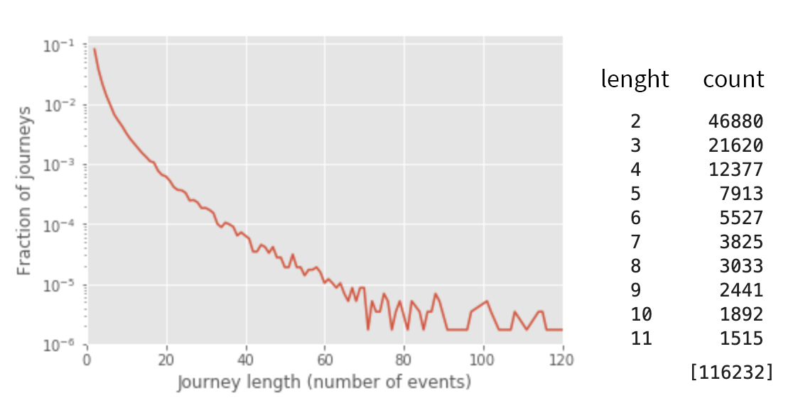
The number of journeys with several events is considerable; thus, it makes sense to try methods for sequential data.

Baseline: Last-Touch Attribution

The most basic and commonly used approach to attribution is position-based models. These models do not use any statistical analysis, but straightforwardly assign the credit to touchpoints based on their position in the journey. The most commonly used options include:

• Last-touch attribution: gives all credit to the last touchpoint in the journey; other touchpoints get zero credit.
• Time-decay attribution: gives more credit to the touchpoints that are closer in time to the conversion.
• Linear attribution: gives equal credit to all touchpoints in the journey.
• U-shaped attribution: gives most of the credit to the first and last touchpoints, and some credit to intermediate touchpoints.
• First-touch attribution: gives all credit to the first touchpoint in the journey.

These models do not really aim to assess the true contribution of touchpoints, but rather encode several different marketing strategies and reallocate budgets according to them. For example, a marketer can choose last-touch attribution to focus resources on customers who already are close to conversion, or first-touch attribution to focus on growth and acquisition. Other models correspond to more balanced strategies.

Last-touch attribution (LTA) is one of the most commonly used options, so we choose to implement it as a baseline. The implementation is quite straightforward:

Click to expand the code sample (21 lines)

def last_touch_attribution(df):
    
    # count the number of events for each campaign in df
    def count_by_campaign(df):                         
        counters = np.zeros(n_campaigns)
        for campaign_one_hot in df['campaigns'].values:
            campaign_id = np.argmax(campaign_one_hot)
            counters[campaign_id] = counters[campaign_id] + 1
        return counters
        
    # count the number of impressions for each campaign
    campaign_impressions = count_by_campaign(df)       
    
    # count the number of times the campaign is the last touch before the conversion
    dfc = df[df['conversion'] == 1]
    idx = dfc.groupby(['jid'])['timestamp_norm'].transform(max) == dfc['timestamp_norm']
    campaign_conversions = count_by_campaign(dfc[idx])
        
    return campaign_conversions / campaign_impressions

lta = last_touch_attribution(df6)

The ratio between the number of journeys in which a given campaign is the last event and the total number of events for the same campaign gives the attribution weight (which can be interpreted as the return per impression). The following chart shows LTA-based weights for a sample of 50 campaigns:

Baseline: Logistic Regression Model

The second baseline model that we build is a simple logistic regression model.^[2] Unlike position-based models, regression analysis aims to reveal touchpoints’ true contributions.

The idea of a regression-based approach is straightforward: Each journey is represented as a vector in which each campaign is represented by a binary feature (and can be other event features), a regression model is fit to predict conversions, and the resulting regression coefficients are interpreted as attribution weights.
The input data we prepared can be thought of as a 3D tensor, in which each event is represented by a vector of features, events are stacked into journeys, and journeys are stacked into the full dataset. We choose simply to aggregate all events in a journey, then fit a model using these aggregates as inputs:

The aggregation strategy depends on a feature: One-hot encoded event features (campaigns and categories) are aggregated into many-hot vectors, in which the number of clicks and costs are summed up. This featured engineering piece and the train-test split are implemented in the code snippet below.

Click to expand the code sample (25 lines)

def features_for_logistic_regression(df):

    def pairwise_max(series):
        return np.max(series.tolist(), axis = 0).tolist()
    
    aggregation = {                      # aggregation specification for each feature
        'campaigns': pairwise_max,
        'cats': pairwise_max,
        'click': 'sum',
        'cost': 'sum',
        'conversion': 'max'
    }
    
    df_agg = df.groupby(['jid']).agg(aggregation)
    
    df_agg['features'] = df_agg[['campaigns', 'cats', 'click', 'cost']].values.tolist()
    
    return (
        np.stack(df_agg['features'].map(lambda x: np.hstack(x)).values),
        df_agg['conversion'].values
    )

x, y = features_for_logistic_regression(df6) 
x_train, x_test, y_train, y_test = train_test_split(x, y, test_size = 0.20)            # train-test split
x_train, x_val, y_train, y_val = train_test_split(x_train, y_train, test_size = 0.20)  # train-validation split

Next, we implement a logistic regression model. We use Keras for consistency with the more complex models developed in the next sections:

m = np.shape(x)[1]
    
model = Sequential()  
model.add(Dense(1, input_dim = m, activation = 'sigmoid', name = 'contributions')) 

model.compile(optimizer='rmsprop', loss='binary_crossentropy', metrics=['accuracy']) 
model.fit(x_train, y_train, batch_size=128, epochs=10, validation_data=(x_val, y_val)) 
score = model.evaluate(x_test, y_test) 
print('Test score:', score[0]) 
print('Test accuracy:', score[1])

#---------

Test score: 0.3732171668471283
Test accuracy: 0.8457783278327833

We are getting reasonably good accuracy for such a basic approach. It is common to assume that attribution weights are non-negative, so let us remap the regression coefficients to non-negative weights using softmax:

from sklearn.utils.extmath import softmax

keras_logreg = model.get_layer('contributions').get_weights()[0].flatten()[0:n_campaigns]
keras_logreg = softmax([keras_logreg]).flatten()

We can compare these weights with the LTA weights computed in the previous section:

The attribution weights produced by two models are highly correlated, although significant differences exist with some campaigns.

We used a relatively simple model design that can be improved through more elaborate feature engineering and aggregation (e.g., one can try to add one-hot encoded event dates). However, advanced feature engineering is generally time consuming and fragile. On the other hand, we can expect to improve the model’s quality and even reduce the feature engineering effort by using methods that can consume sequences of events directly, i.e., without any aggregation. We explore this idea in the next two sections.

LSTM Model

Our next step is to build a more advanced model that explicitly accounts for dependencies between the events in a journey. This problem can be framed as a conversion prediction based on the ordered sequence of events, and recurrent neural networks (RNNs) are a common solution for it. We choose to use a basic long short-term memory (LSTM) architecture with 64 hidden units, as illustrated in the figure below (hereafter, blue arrows denote fully connected layers):

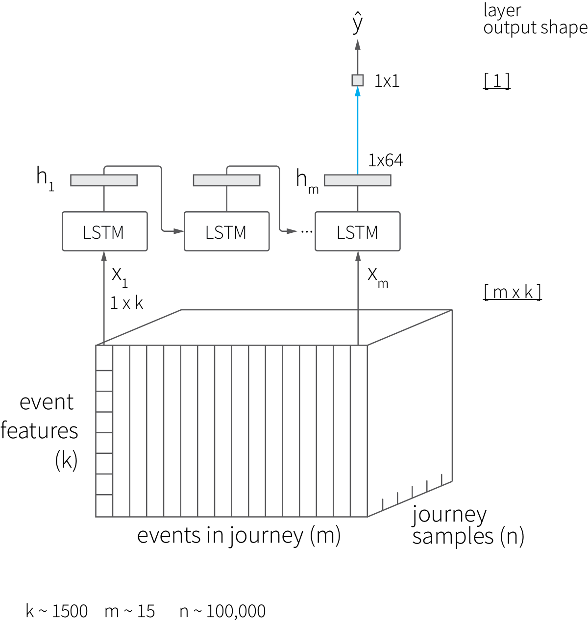
The LSTM-based approach does not require the feature aggregation that we used for the logistic regression model, but we need to pack the events into a 3D tensor, as shown in the figure above. The implementation of this data repackaging is shown in the following code snippet.

Click to expand the code sample (38 lines)

def features_for_lstm(df, max_touchpoints):
    
    df_proj = df[['jid', 'campaigns', 'cats', 'click', 
                  'cost', 'time_since_last_click_norm', 'timestamp_norm', 'conversion']]
    
    x2d = df_proj.values
    
    # group events by JID
    x3d_list = np.split( x2d[:, 1:], np.cumsum(np.unique(x2d[:, 0], return_counts=True)[1])[:-1])
    
    x3d = []
    y = []
    for xi in x3d_list:
        journey_matrix = np.apply_along_axis(np.hstack, 1, xi)
        
        # sort events by timestamp
        journey_matrix = journey_matrix[ journey_matrix[:, 5].argsort() ]   
        
        # truncate long journeys or add zero event vectors to short journeys 
        # so that all journeys have lenght of max_touchpoints 
        n_touchpoints = len(journey_matrix)
        padded_journey = []
        if(n_touchpoints >= max_touchpoints):
            padded_journey = journey_matrix[0:max_touchpoints]
        else:
            padded_journey = np.pad(journey_matrix, 
                                    ((0, max_touchpoints - n_touchpoints), (0, 0)), 
                                    'constant', constant_values=(0))
            
        x3d.append(padded_journey[:, 0:-1])
        y.append(np.max(padded_journey[:, -1]))
        
    return np.stack(x3d), y

x, y = features_for_lstm(df6, max_touchpoints = 15)                                    # truncate journeys to 15 events

x_train, x_test, y_train, y_test = train_test_split(x, y, test_size = 0.20)            # train-test split 
x_train, x_val, y_train, y_val = train_test_split(x_train, y_train, test_size = 0.20)  # train-validation split

The model can be implemented, fitted, and evaluated straightforwardly using Keras as follows:

from keras.models import Sequential 
from keras.layers import Dense, LSTM

n_steps, n_features = np.shape(x)[1:3]
    
model = Sequential() 
model.add(LSTM(64, dropout=0.2, recurrent_dropout=0.2, input_shape=(n_steps, n_features)))
model.add(Dense(1, activation='sigmoid')) 

model.compile(optimizer='rmsprop', loss='binary_crossentropy', metrics=['accuracy']) 
model.fit(x_train, y_train, batch_size=64, epochs=5, validation_data=(x_val, y_val)) 
score = model.evaluate(x_test, y_test) 
print('Test score:', score[0]) 
print('Test accuracy:', score[1])

#---------

Test score: 0.21668663059081575
Test accuracy: 0.9088627612761276

We can see that the LSTM approach provided significantly better accuracy compared with the logistic regression baseline. However, LSTM does not provide a simple way to extract the attribution weights from the fitted model. Fortunately, we can build a much better model on top of LSTM that provides both better accuracy and explicit estimates of attribution weights.

LSTM with Attention

The LSTM model described in the previous section starts with a random hidden state vector $h$, sequentially updates it after each input event, and estimates the conversion probability based on the hidden vector’s final state. This approach is known to be limited in the sense that the hidden vector’s final state is not always the best representation of the sequence, and better results can be obtained by using the weighted average of the hidden vector’s intermediate states:

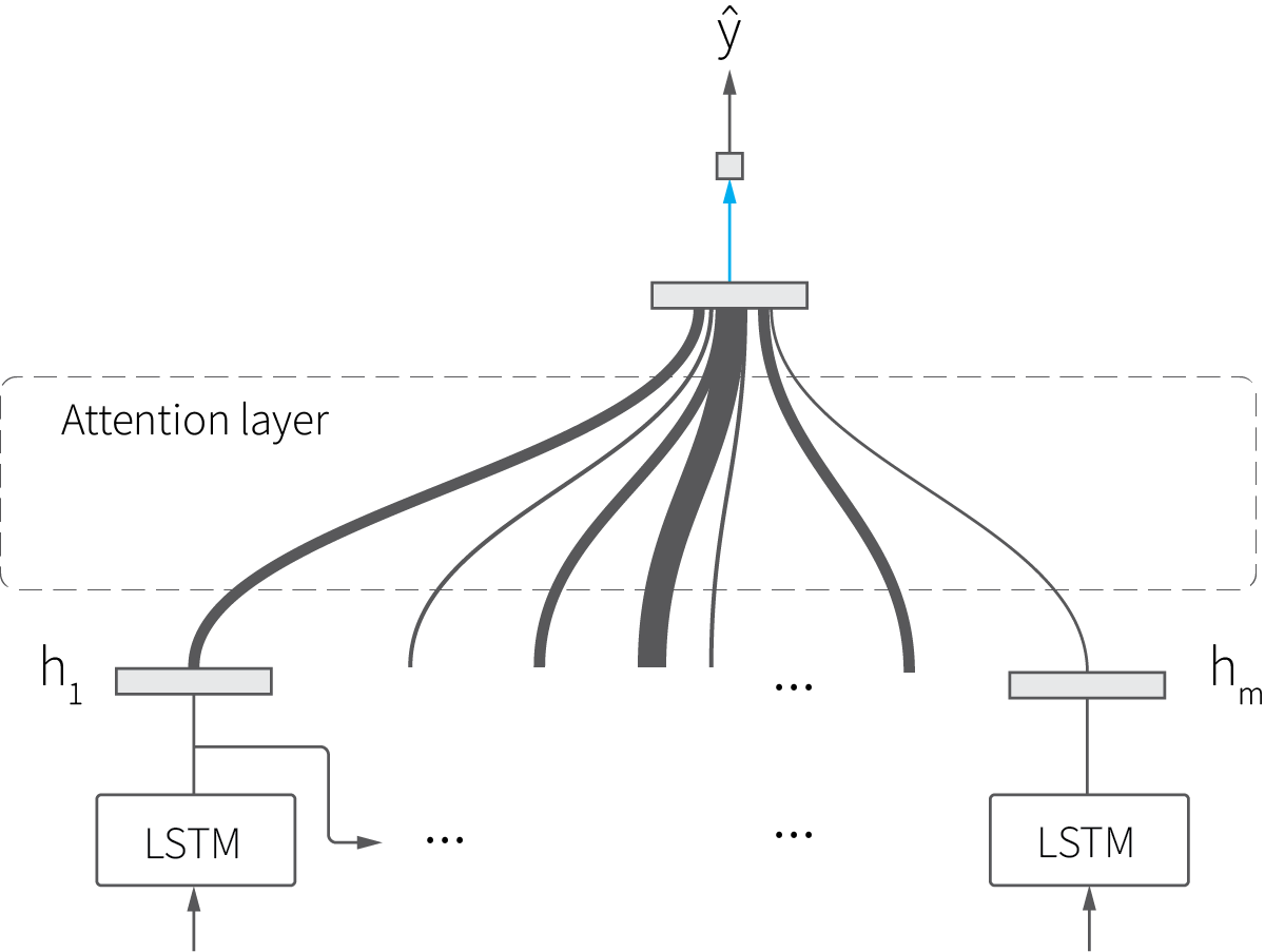
This extension of a basic RNN is known commonly as an attention mechanism. It originally was developed for natural language processing (NLP) applications in which the intuition was that the weights associated with the intermediate states essentially model attention that a human reader pays to different words in a sentence.^[3] The attention mechanism is known to be very efficient for sequence modeling in general, and several attention-based models recently were proposed specifically for the attribution problem, so we implement a variant of the attention-based model in this section.^[4][5]

First, let us briefly review the design of the attention mechanism. As we already mentioned, the main idea is to learn the attention weights that can be used to combine the intermediate hidden vectors $h_t$ together. Thus, attention weights can be interpreted as amplifiers that control the contribution of individual hidden vectors in the final vector $s$, which is used to make the prediction. A typical implementation of the attention mechanism includes the following operations:

• First, a fully connected layer with $\text{tanh}$ activation is used to squash each hidden vector $h_t$ into an attention vector $u_t$:

$$
u_t = \tanh(W \ h_t + b)
$$

• Second, the importance of each event (attention weight) is estimated as a normalized similarity between $u_t$ and a so-called context vector $c$ that is learned jointly during the fitting process:

$$
a_t = \text{softmax}(u_t^T \ c )
$$

• Finally, the journey vector $s$ is obtained as an attention-weighted sum of the hidden vectors:

$$
s = \sum_t a_t h_t
$$

We choose to use a slightly simplified variant of the above design, in which $u_t$ is scalar; thus, context vector $c$ is redundant. Finally, we add a linear embedding layer in front of the LSTM layer to map sparse one-hot encoded event vectors to more dense 128-dimensional even embeddings, as suggested in ^[4:1]. This overall model design is shown in the diagram below.

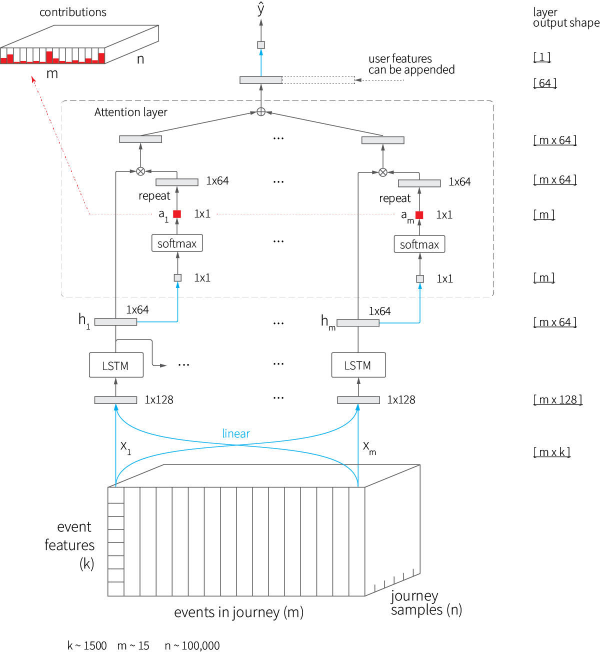
Note that the feature vector produced by the top layer of the model can be augmented with additional journey-level features such as customer demographics. The implementation of this model in Keras is quite straightforward:

n_steps, n_features = np.shape(x)[1:3]
hidden_units = 64

main_input = Input(shape=(n_steps, n_features))
    
embeddings = Dense(128, activation='linear', input_shape=(n_steps, n_features))(main_input)

activations = LSTM(hidden_units, dropout=0.2, recurrent_dropout=0.2, return_sequences=True)(embeddings)

attention = Dense(1, activation='tanh')(activations)
attention = Flatten()(attention)
attention = Activation('softmax', name = 'attention_weigths')(attention)
attention = RepeatVector(hidden_units)(attention)
attention = Permute([2, 1])(attention)

weighted_activations = Multiply()([activations, attention])
weighted_activations = Lambda(lambda xin: K.sum(xin, axis=-2), 
                              output_shape=(hidden_units,))(weighted_activations)

main_output = Dense(1, activation='sigmoid')(weighted_activations)

model = Model(inputs=main_input, outputs=main_output)

# training and evaluation like for LSTM

# ---------

Test score: 0.19408383931476947
Test accuracy: 0.9186262376237624

The attention mechanism clearly improves the accuracy of the model, but it also provides a convenient way to estimate attribution weights: We can just take the values of the attention vectors for each journey and average them across all training samples. This piece is highlighted in the above model design diagram in red.

Keras allows for cutting a trained model’s head and making predictions with a truncated model, so that the output is not the final conversion probability, but rather the output of a hidden layer, which is an attention layer in our case. We do this in the implementation below, i.e., build a truncated model, run predictions for all journeys in a training set, then compute average attention weights for each campaign:

def get_campaign_id(x_journey_step):
    return np.argmax(x_journey_step[0:n_campaigns])

# truncated model that outputs attention weights
attention_model = Model(inputs=model.input,    
                        outputs=model.get_layer('attention_weigths').output)

# compute attention vectors for each journey
a = attention_model.predict(x_train)      

# average attention weights across all journeys
attributions = np.zeros(n_campaigns)
campaign_freq = np.ones(n_campaigns)
for i, journey in enumerate(a):
    for t, event_contribution in enumerate(journey):
        if(np.sum(x_train[i][t]) > 0):
            campaign_id = get_campaign_id(x_train[i][t])
            attributions[campaign_id] = attributions[campaign_id] + event_contribution
            campaign_freq[campaign_id] = campaign_freq[campaign_id] + 1

lstm_a = attributions/campaign_freq   # final attribution weights

This produces attribution weights similar to the previous models:

These weights generally are correlated with the baseline LTA weights:

It is important that the attention weights in each journey are not independent, but that each weight quantifies the contribution of a touchpoint, given all other touchpoints in the journey, so that subsequences (pairs, triplets, etc.) of campaigns also can be analyzed.

Budget Optimization

We have produced four different sets of attribution weights using four different models. Each of these sets can be used directly to reallocate the budget, but how do we tell which one promises the best return on investment (ROI)? We simply can assume that the higher-accuracy models produce better weights, but it would be a good idea to validate this assumption. One possible way to facilitate this validation is to simulate campaign execution under the new budgeting constraints by replaying historical events.^[5:1]

The campaign simulation idea can be outlined as follows:

• At the beginning of the process, we distribute a limited budget across the campaigns according to the attribution weights.
• We replay the available historical events (ordered by their timestamps) and decrement the budgets accordingly.
• Once a campaign runs out of money, we stop to replay the remaining events associated with it and somehow estimate the probabilities of conversion for all journeys affected by this campaign’s suppression.
• Finally, we count the total number of conversions and estimate ROI. If none of the campaigns in a converted journey runs out of money before the journey ends, this conversion will be counted explicitly. Otherwise, the estimate of the conversion probability will be used.

We implement this approach using two simplifying assumptions. First, we define the budget just as the number of events (impressions) that we can pay for, ignoring actual dollar costs. Second, we assume that once a campaign runs out of money, all journeys that have more events associated with this campaign will never convert. These assumptions lead to the following simulation algorithm:

This algorithm’s implementation is shown in the code snippet below.

def simulate_budget_roi(df, budget_total, attribution, verbose=False):
    # convert attribution weights to budgets
    budgets = np.ceil(attribution * (budget_total / np.sum(attribution)))  
    
    blacklist = set()
    conversions = set()
    for i in range(df.shape[0]):                                  # simulation loop
        campaign_id = get_campaign_id(df.loc[i]['campaigns']) 
        jid = df.loc[i]['jid']
        if jid not in blacklist:
            if budgets[campaign_id] >= 1:
                budgets[campaign_id] = budgets[campaign_id] - 1
                if(df.loc[i]['conversion'] == 1):
                    conversions.add(jid)
            else:
                blacklist.add(jid)
            
    return len(conversions.difference(blacklist))

This simulation algorithm can be used to evaluate the performance of the original attribution weights produced by the models, as well as various transformations of these weights. For example, we can evaluate not only the original weights $w$, but also weights $w^p$ for different values of parameter $p$. This parameter essentially controls the "pitch" of the budget distribution: The values of $p$ between zero and one lead to a more even distribution of the budget across the campaigns; the values higher than one lead to a more uneven distribution:

The results of the simulation indicate that the raw attribution weights ($p=1.0$) are not necessarily optimal for all models:

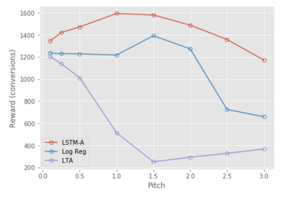
These results also confirm that LSTM with attention provides the best budget allocation, and that logistic regression performs reasonably well with a properly selected pitch value. LTA has very poor performance because it focuses exclusively on the campaigns at the end of the journey, so the campaigns at the beginning of the journey quickly run out of money, sending these journeys to the blacklist.

The simulation algorithm can be extended straightforwardly to incorporate the events’ costs, conversion profits, or more sophisticated logic for handling out-of-budget journeys. These adjustments can be designed and fine-tuned based on the actual performance of the optimized budgets in production.

Conclusions

We have discussed, implemented, and evaluated several attribution models that provide a solid foundation for measuring the efficiency of marketing activities and the optimization of budgeting parameters. We have seen that the state-of-the-art models that consume sequences of events provide superior accuracy and greatly simplify feature engineering. In fact, this is a typical example of how traditional enterprise data science can benefit from deep and reinforcement learning: Many marketing, merchandising, and supply-chain use cases deal with sequential data or multi-step optimization, and deep and reinforcement learning provide powerful toolkits for these types of problems. Other examples of that kind include next best action modeling, demand prediction, and inventory-constrained price optimization, to name a few.

We generally assumed availability of historical data for modeling and optimization. However, the same techniques can be combined with reinforcement learning to evaluate and adjust budgeting parameters dynamically. This approach can be particularly useful for sponsored search bids optimization and other use cases in which a large number of budgeting parameters needs to be tuned dynamically. ^[6]

A complete notebook with the data preparation code and models is available on github.

Resources

---

1. http://ailab.criteo.com/criteo-attribution-modeling-bidding-dataset/ ↩︎

2. Shao X. and Li L., Data-Driven Multi-Touch Attribution Models, 2011. ↩︎

3. Bahdanau D., Cho K., and Bengio Y., Neural Machine Translation by Jointly Learning to Align and Translate, 2014. ↩︎

4. Li N. et al., Deep Neural Net with Attention for Multi-Channel Multi-Touch Attribution, 2018. ↩︎ ↩︎

5. Ren K., Fang Y., Zhang W., Liu S., Li J., Zhang Y., Yu Y., and Wang J., Learning Multi-Touch Conversion Attribution with Dual-Attention Mechanisms for Online Advertising, 2018. ↩︎ ↩︎

6. Zhao J., Qiu G., Guan Z., Zhao W., and He X., Deep Reinforcement Learning for Sponsored Search Real-Time Bidding, 2018. ↩︎