Customer2Vec: Representation learning for customer analytics and personalization

Personalization and recommendation algorithms have been around for many decades, and basic methods such as look-alike modeling and collaborative filtering are widely understood and adopted across the industry. The advancement of deep learning greatly expands the toolkit available to developers of personalization solutions as it offers simpler feature engineering, higher predictive accuracy, and more flexible model architectures.

In this article, we focus on the learning of useful semantic representations (embeddings) for products and customers using neural networks. These representations can be used for multiple purposes: they can be utilized as features in downstream models to improve the accuracy of propensity scores and recommendations, they can be used to cluster and analyze embeddings to gain deep insights into the semantics of customer behavior, or they can be used to perform other personalization and analytics tasks that use embeddings to measure the proximity between products and customers. These approaches generally outperform standard segmentation and personalization methods, which use demographic attributes and hand-crafted behavioral features.

We show that many of these representation learning tasks can be efficiently accomplished using standard natural language processing (NLP) methods. We describe exactly how customer analytics and personalization problems can be related to NLP problems and show how representation learning models for products and customers (so-called item2vec and customer2vec) can be derived directly from their NLP counterparts, such as word2vec and doc2vec. This article is structured as follows:

• In the first section, we briefly survey traditional personalization methods and discuss their limitations and problems. Readers who are familiar with traditional approaches can just skim this section.
• In the second section, we discuss how item2vec and customer2vec approaches overcome the limitations of traditional methods, and we present several case studies of how these models were implemented in practice.
• In the last section, we present a hands-on tutorial on how to train and analyze item2vec and customer2vec models using a public dataset of Instacart orders. The corresponding notebooks are available on GitHub as part of the TensorHouse project.

Limitations of Traditional Personalization Methods

The most common categories of personalization models that are traditionally used in the industry are look-alike modeling, collaborative filtering, content-based filtering, and demographic segmentation. First, let us take a close look at the first two approaches and their limitations.

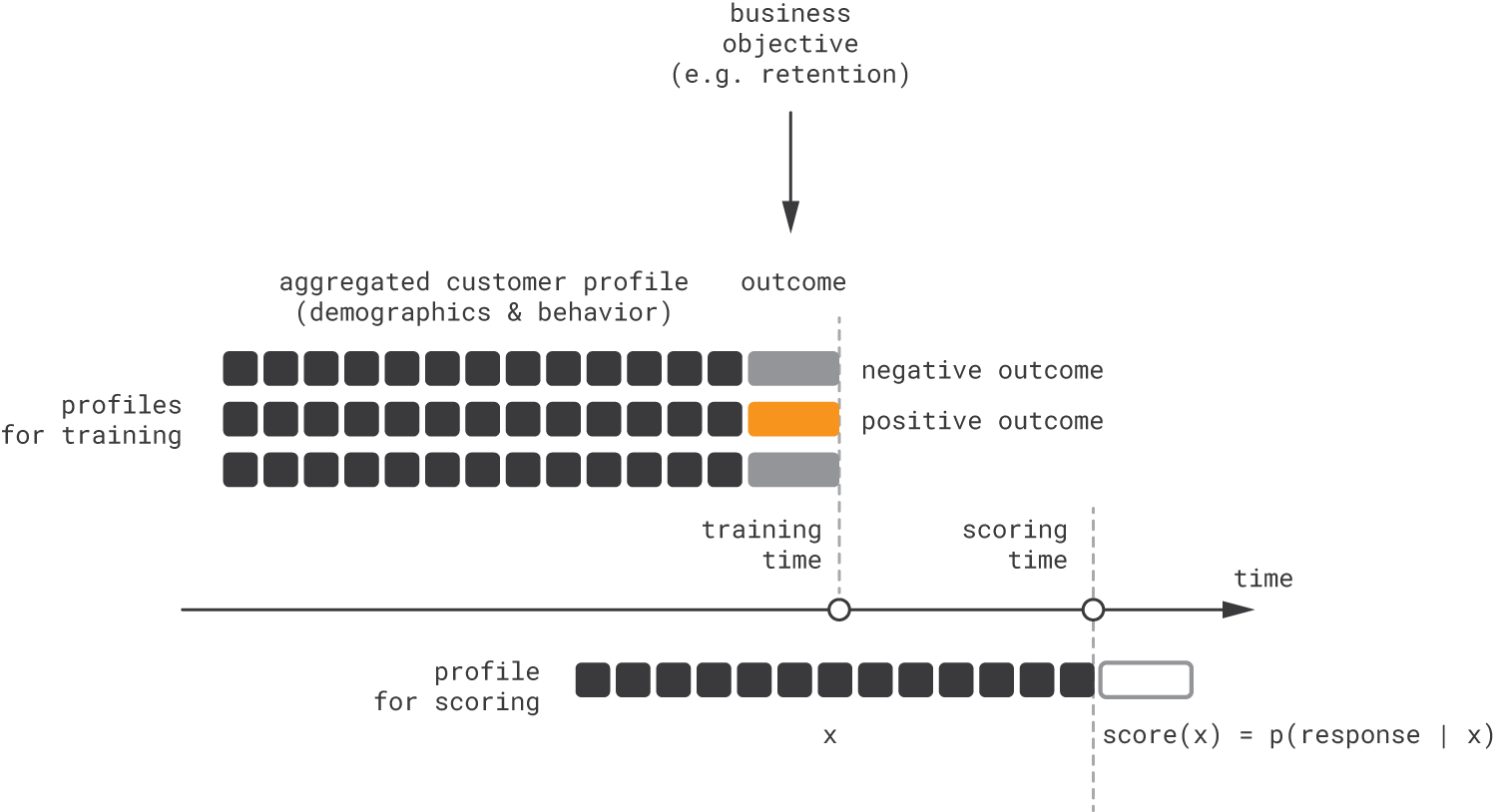
The look-alike approach is focused on building regression or classification models that identify individuals who appear to be similar to the target audience. The modeling process typically includes hand-engineering of customer features based on demographic and behavior data, engineering of target labels based on the definition of the target audience (i.e., good targets for customer acquisition, retention, or some other objective), and model training based on a collection of historical profiles, as shown in the figure below.

For product recommendations, we need to predict outcomes not only for customers but also for product–customer pairs in order to rank items in a personalized context. Conceptually, this can be accomplished by extending the feature vector with one-hot item encodings, as illustrated below.

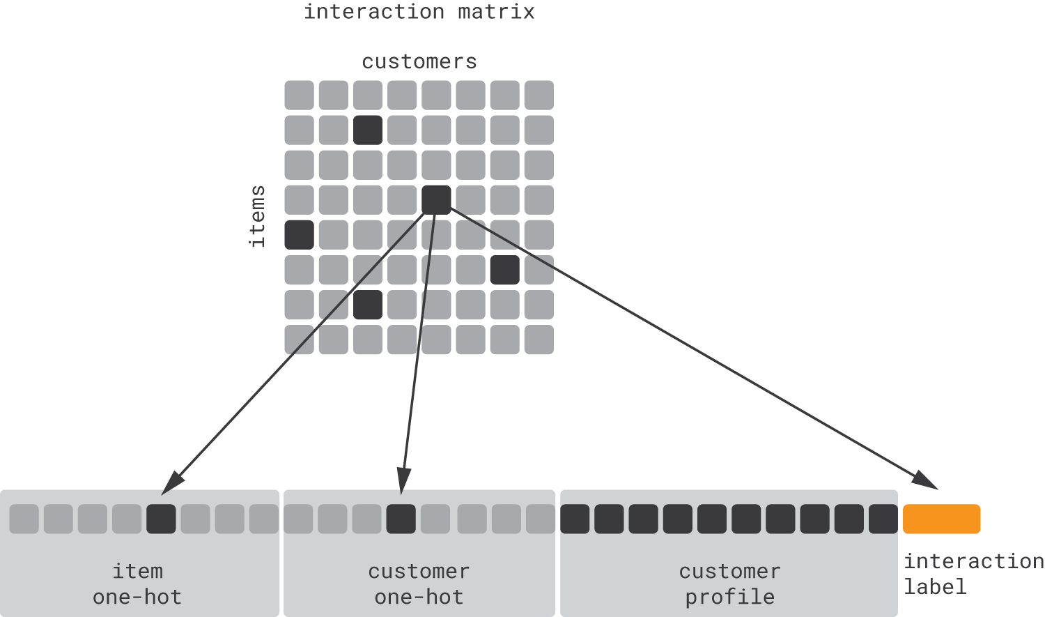
Note that the above schema is effectively a definition of collaborative filtering. Fitting a classification or regression model with such sparse features, however, requires using dimensionality reduction techniques rather than generic classification methods. Thus, it is more common to view collaborative filtering as a matrix completion problem (which corresponds to the upper part of the figure) and to apply matrix factorization or other specialized methods. Nevertheless, due to the close relationship between look-alike modeling and collaborative filtering, they share many common limitations:

• Hand-crafted features. The accuracy of a look-alike model completely depends on the quality of customer features that need to be manually engineered. Likewise, collaborative filtering requires the developer to make many design decisions regarding the interaction matrix and objective function [Koren09]. Manual feature engineering is known to be one of the biggest challenges in industrial machine learning; it requires domain knowledge, time-consuming experimentation for every use case, and continuous curation and update efforts. Additionally, it has limited scalability because models cannot be automatically created and maintained. The problem becomes particularly challenging when raw data come not from well-structured sources, such as a customer master data management (MDM) platform, but from application logs, which are often poorly documented and volatile and have sophisticated or imperfect field semantics [Seleznev18].
• Aggregation of event sequences. Fundamentally, a customer behavior profile is a sequence of events (page views, clicks, purchases, etc.), but traditional machine learning methods require fixed-length input feature vectors. This mismatch is traditionally resolved by collapsing event sequences into aggregated features, such as averages and totals. However, this approach tends to lose information about temporal dependencies between events. In theory, much of this information can be preserved through careful feature engineering, but it represents a major practical challenge, as we discussed above.
• Disconnect from content data. Historically, behavior- and content-based personalization methods evolved in parallel. There are different ways that look-alike modeling and collaborative filtering can be integrated with content-based methods to develop a hybrid solution, but it is intuitively clear (and proven in practice) that deep learning allows for more efficient personalization model architectures that derive and combine embeddings from behavioral, textual, and image data in a unified way. Moreover, some useful data sources, such as graphs of financial transactions, that did not receive adequate attention in the context of traditional personalization methods are now being unlocked with the advent of deep graph learning and other new methods.
• Reliance on historical data. Traditional methods require historical data for model training, and they assume a relatively static environment in which patterns learned from past observations are relevant for optimization of future actions. These two prerequisites might not be present in dynamic environments in which new content items (short-term deals, new products, or news posts) are frequently deployed.
• Focus on myopic optimization. Traditional personalization models are usually designed to optimize an immediate action and its outcome (e.g., which banner maximizes the click-through rate). In most settings, however, the ultimate goal is to jointly optimize the sequence of actions (recommendations, offers, or notifications) in a way that improves long-term customer engagement.

These considerations are summarized in the figure below.

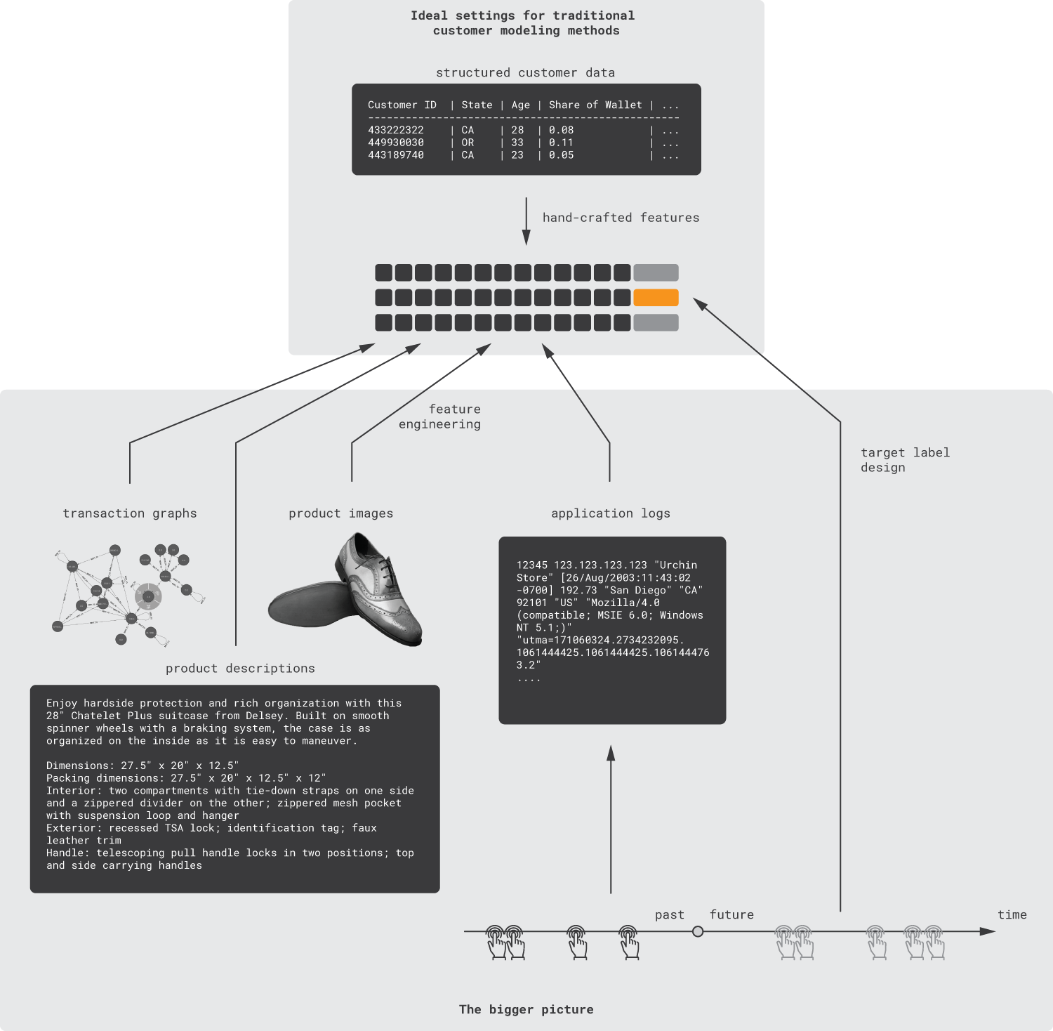
In this article, we will focus on the first three issues outlined above and develop a toolkit that helps to reduce the effort required for feature engineering, account for event sequences, and incorporate a wide range of data types. The last two problems can be addressed using reinforcement learning methods, but this side of the problem is beyond the scope of this article.

Next, let us return to the other two basic methods we mentioned at the beginning of this section: customer segmentation and content-based filtering. Customer segmentation with basic clustering algorithms is prone to the same issues: the feature space needs to be manually designed, events are aggregated, and content data are not easy to incorporate. Content-based filtering helps to incorporate content data, but integration of these methods with behavioral methods is another challenge to overcome.

Theory and Models

In this section, we develop a toolkit of methods for learning useful representations from customer data. These representations can be used for customer behavior analysis or as features or distance metrics for downstream personalization models.

We start with the most basic methods and gradually move to more advanced methods. Also, we focus on concepts and do not deeply discuss aspects of implementation until the next section.

Step 1: Learn from Event Sequences Using RNNs

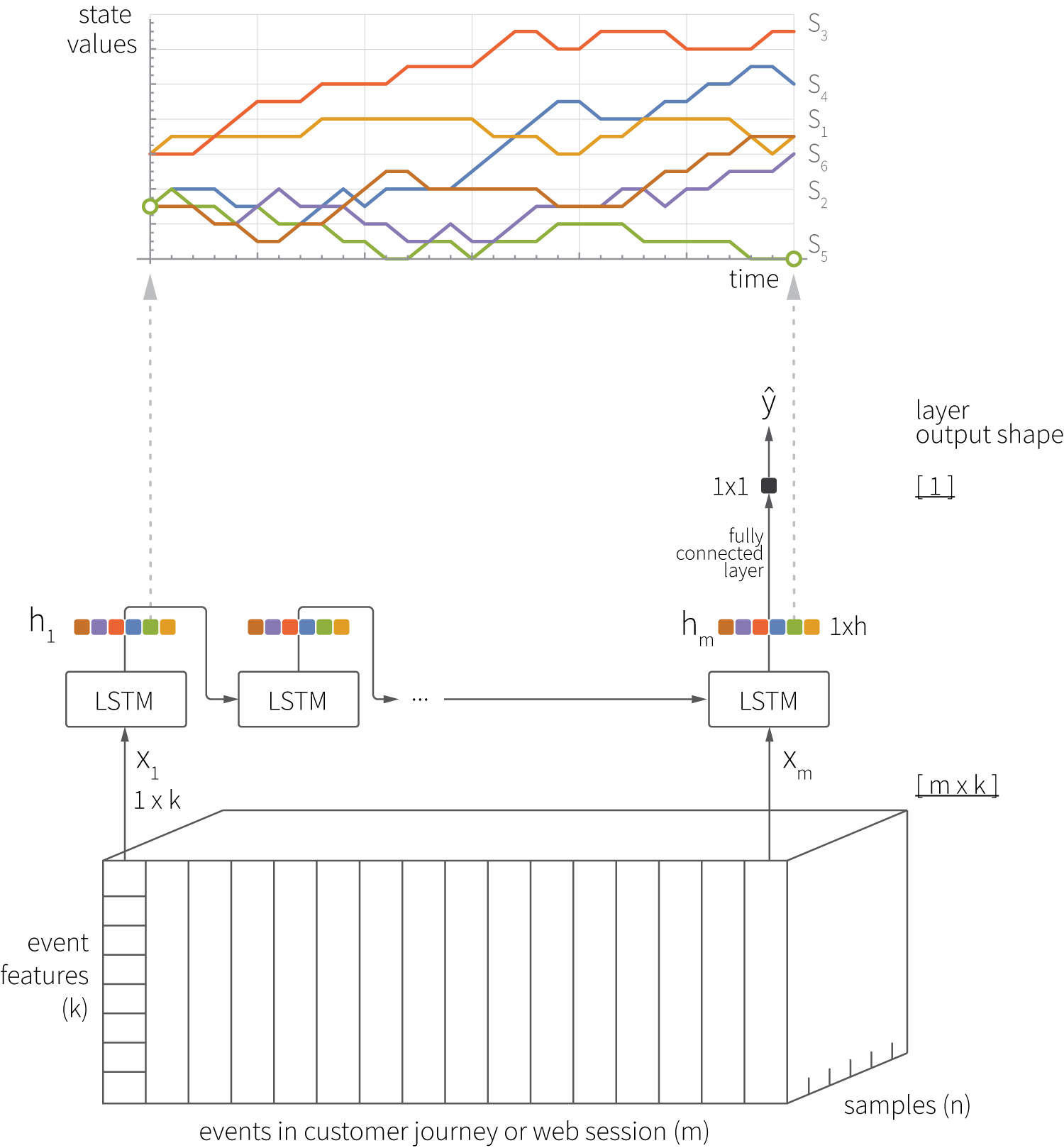
One of the most straightforward solutions for modeling customer journeys at the level of individual events is recurrent neural networks (RNNs). Customer journeys can be naturally represented as sequences of events, and each event is modeled as a vector of event-level features. This input can be directly consumed by an RNN, and the network can be trained to predict some outcomes, such as a conversion event or the ID of the products that are clicked on next ($\hat{y}$ in the figure below).

This approach offers the following advantages:

• The accuracy of such models is generally higher than the accuracy of models that use aggregated features. Many companies reported that LSTM- or GRU-based approaches can be applied to a variety of use cases, including churn prediction, conversion prediction, and product recommendations, with consistently good results [Hidasi16, Zolna16, Lang17, Yang18].
• The RNN-based approach reduces the complexity of feature engineering by replacing customer-level features with event-level features. It is much easier to design event features than design aggregates that summarize an entire customer history, including all important behavioral and demographic characteristics.
• The RNN-based approach can successfully learn from short event sequences such as web sessions, as many sessions have only 2–3 events. This makes the RNN-based approach efficient in contexts like session-based recommendations, for which complex collaborative filtering methods like factor models are not applicable and more basic methods, like nearest neighbors, are not especially accurate [Hidasi16].
• Finally, and most importantly for this article, hidden LSTM states can be interpreted as customer embeddings. For instance, the above illustration shows how the values of individual elements of the state vector are traced over time, and these traces can be compared with the trace of the predicted metric [Zolna16]. In this way, one can identify latent dimensions that are correlated with, for example, the probability of conversion.

Step 2: Learn Product Embeddings Using NLP Methods

Over the last few years, deep learning methods in the field of NLP have advanced tremendously from generic RNNs to highly specialized architectures like BERT. In the field of customer intelligence, one can significantly benefit from these advancements by recognizing that customers, sessions, and orders can be thought of as texts.

As an introductory example, consider a database of customer orders in which each order typically includes multiple products (e.g., a grocery business). We can interpret each order as a sentence and each product as a word and straightforwardly apply the standard word2vec model to learn product embeddings, as shown below.

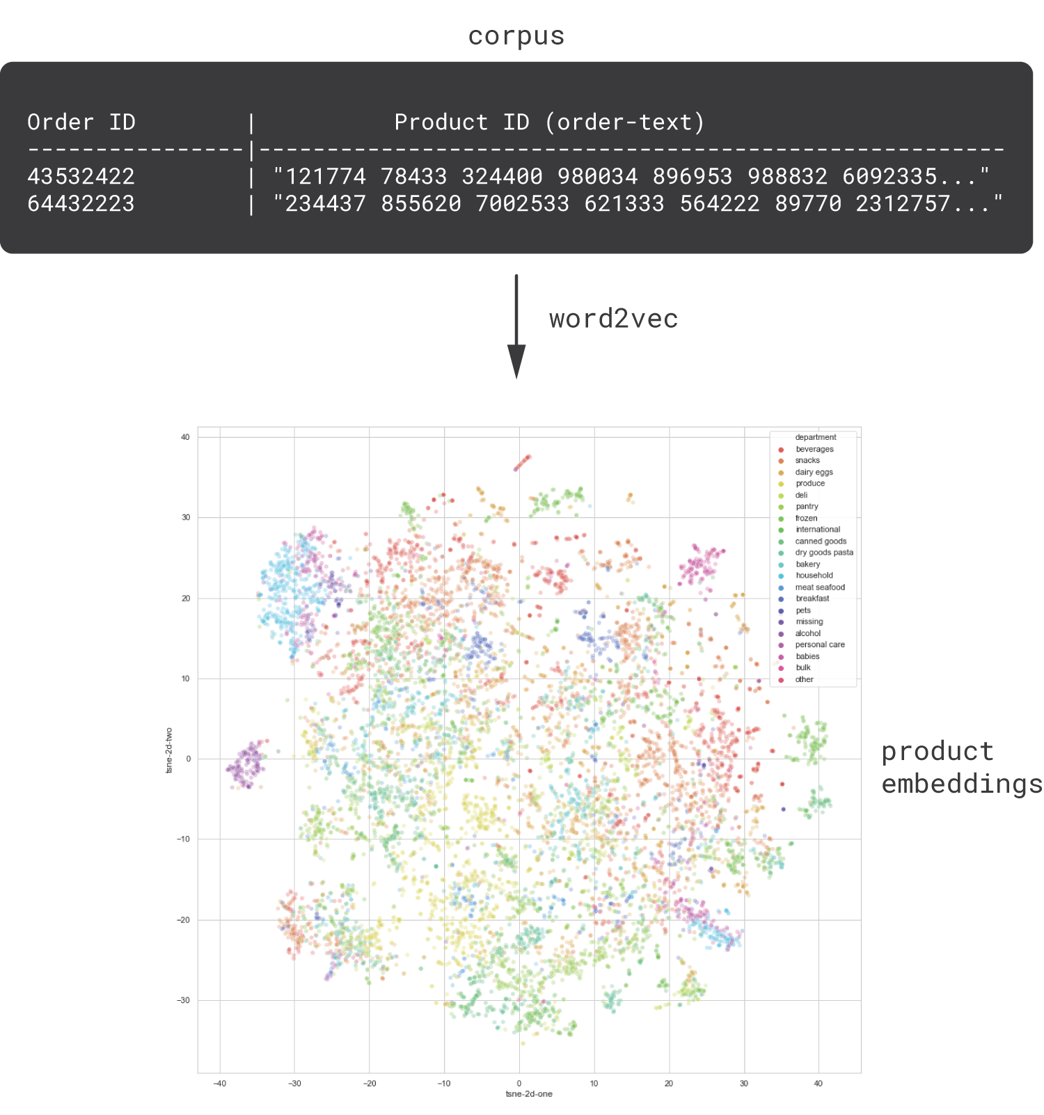
This type of models is known as item2vec [Barkan2016]. This simple approach is known to produce useful product embeddings that capture purchasing or browsing patterns and reveal the affinity between products that are perceived or used in similar ways by customers. As we will see in the hands-on section, these embeddings are generally aligned with canonical product categorizations, such as music genres (in the case of media products) or departments (in the case of a department store).

We thoroughly discuss the usage of embeddings produced in this way in the next section, after we review several possible extensions.

Step 3: Mix Behavioral and Content Features

The beauty of the word2vec approach is that the basic solution described in the previous section can be naturally extended in many ways to incorporate multiple heterogeneous data sources. For example, one can incorporate content data by replacing product IDs with product attributes [Arora16]. In this way, orders or web sessions can be represented as flat sequences of product attributes and then attribute embeddings can be learned.

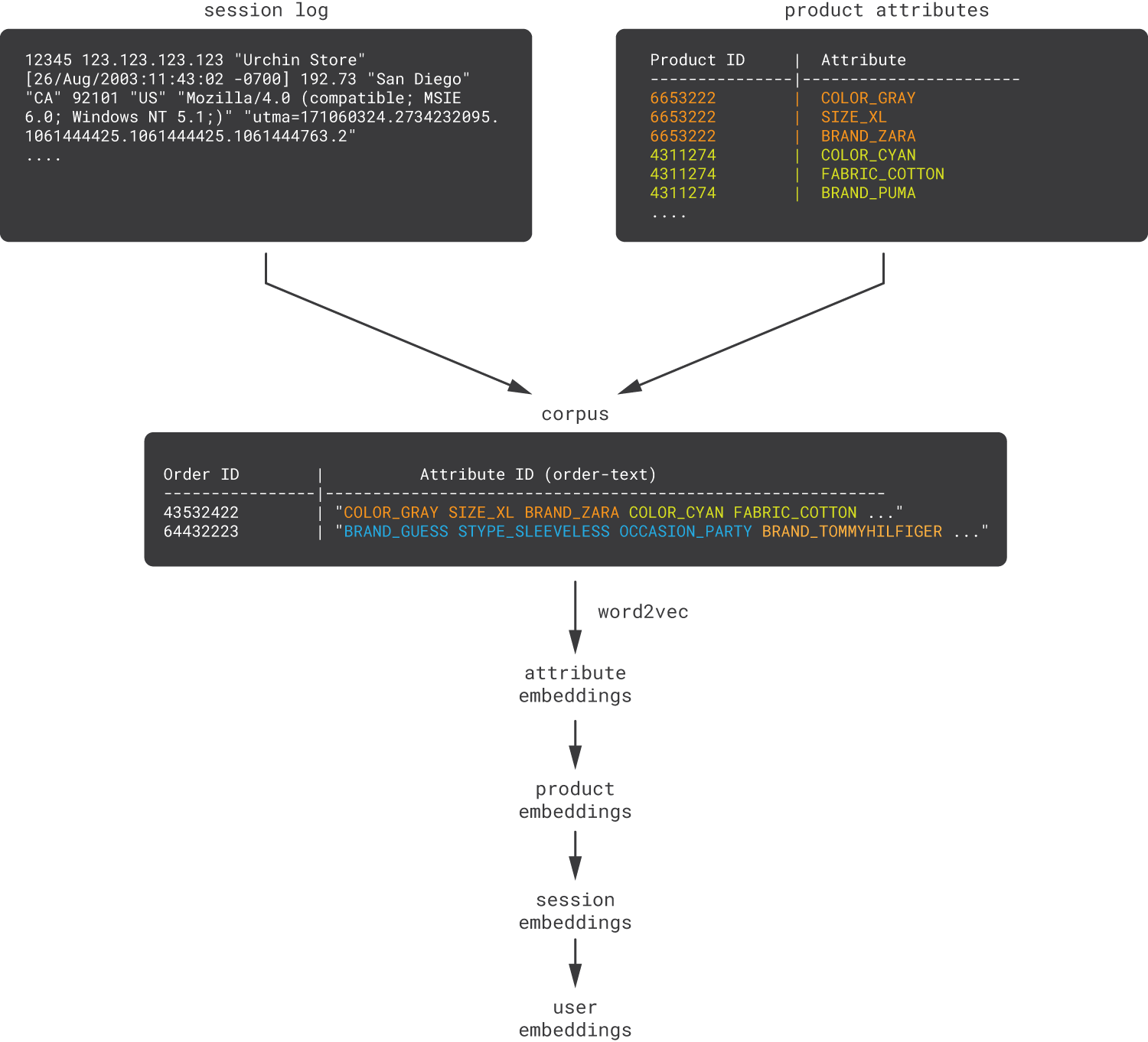
This approach efficiently blends behavioral data with product data, capturing both purchasing patterns and attribute-based product similarities. The obtained attribute embeddings can be rolled up into product embeddings, then session embeddings, and finally customer embeddings. This rolling up process can usually be done through simple averaging (for example, a product embedding is the average of the embeddings of all its attributes).

The above approach can be extended to incorporate even less structured content data. For example, one can replace product attributes with human-readable textual product descriptions (lists of words instead of lists of attributes) if structured attributes are not available or not informative enough, and embeddings can be learned using the same off-the-shelf word2vec algorithm [Stiebellehner17]. Surprisingly, one can obtain very good results this way without dealing with complex feature engineering or fragile relevancy tuning, which are required by traditional hybrid recommendation algorithms.

The embeddings learned using the simple methods discussed above have many usages, including the following:

• Item-to-item recommendations. Product embeddings computed as described in steps 2 or 3 can be used to measure distances between products in the semantic space, and this can be straightforwardly used to build an item-to-item recommender system [Phi16].
• User-to-item recommendations. Embedding roll-up enables computing of customer embeddings, which in turn enables user-to-item recommendations or similar personalization use cases [Phi16, Arora16].
• Contextual recommendations. Consider the following example. A customer who visits an online fashion store might be shopping in several different modes or contexts. She might be looking for a specific product, a specific style, or a certain combination of products, such as socks and shoes. Understanding this context is essential for a personalization system. This can be done by computing session embeddings and then measuring the distance between the session and personalizable items, such as products, in the latent space.
• Automated feature engineering. Item2vec models learn embeddings in an unsupervised way from data that is easy to engineer (i.e., sequences of product IDs), which makes them a good AutoML component that can be integrated with downstream customer models. We develop this idea further in the following sections.
• Analytics and segmentation. Similar to the recommendation and propensity modeling use cases, products and customers can be analyzed and segmented more efficiently in embedding spaces than in spaces of manually engineered features. We explore this thoroughly in the hands-on section.

Step 4: Learn Customer Embeddings

Although the item2vec models described in the previous sections can produce customer embeddings using roll-ups, this is not the only approach. Another natural solution is to use doc2vec instead of word2vec.

Word2vec learns from plain sequences of tokens and uses the notion of a sentence only to reset the learning context. It does not support any hierarchical relationships, such as product–order–customer. This is clearly a limitation because events in a customer journey depend not only on global event patterns but also on customer identities. In the NLP world, an equivalent problem is learning sentence embeddings (as opposed to word embeddings). The standard solution for this problem is doc2vec, which directly generates sentence embeddings. We can straightforwardly adapt doc2vec to learn customer embeddings from customer-sentences. The difference between these two approaches can be clarified as follows:

• Word2vec is based on the idea that word representation should be good enough to predict surrounding words (e.g., “the cat sat on the” predicts “mat”). This makes sense for product representations as well (e.g., “wine cheese” predicts “grapes”).

• Doc2vec is based on the idea that a sentence (i.e., document) representation should be good enough to predict words in the sentence. For example, “the most important → thing” may be the best prediction on average, but “the most important → feature” may be the best prediction for a text on machine learning. Similarly, a good customer embedding should predict future events for this customer. Customer embeddings obtained by averaging the product embeddings associated with customer interaction history do not necessarily achieve this goal.

The following schematic summarizes the doc2vec approach to learning customer embeddings [Phi16, Zolna16]. The main difference between this schema and the designs we presented in steps 2 and 3 is the doc2vec algorithm itself; the algorithm consumes inputs similar to item2vec, but it outputs embeddings for customers (sentences), not products (words).

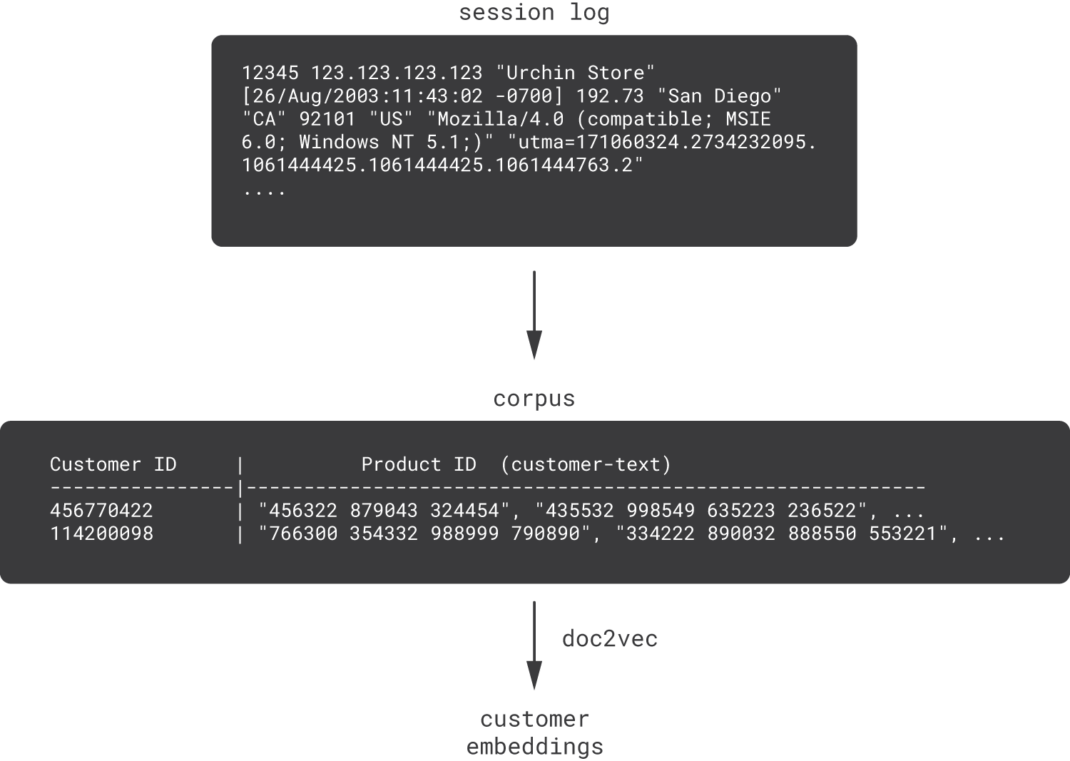
This category of model is commonly referred to as user2vec, client2vec, or customer2vec.

Step 5: Learn Directly from Application Logs

We have seen that the NLP-based approach allows one to blend behavioral and content data in various ways as well as produce embeddings for different levels of aggregation, such as attributes, products, and customers. These embeddings can then be consumed as features by downstream models like conversion propensity or price sensitivity scoring. The quality of embeddings can be so high that it is sometimes possible to completely get rid of manually engineered features and replace them with embeddings that are automatically generated by item2vec or customer2vec models [Seleznev18].

If we look at customer2vec from the AutoML perspective, then we can recognize that the customer-as-a-text paradigm not only helps to combine customer analytics with NLP but also can be taken literally – in many settings, customer data originates in application logs.

For example, consider a website or mobile application that continuously logs events with a timestamp, event type (click, view, etc.), event attribute (page, click coordinates, etc.), and other fields. Consider also a data scientist who is tasked with engineering features for some models out of these log files. In practice, this task can be quite challenging because one needs to thoroughly study log samples, understand the semantics of fields, learn how multiple related events can be stitched together, examine corner cases, and so on. However, one can approach the problem from a different angle: event names and attributes can be automatically concatenated into discrete tokens, tokens can be grouped into customer-sentences, and then customer2vec can be applied [Seleznev18].

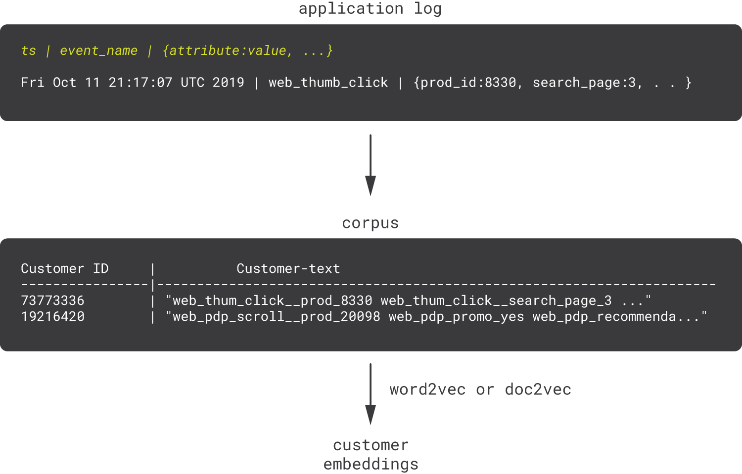
This example shows how customer2vec can simplify not only modeling but also the operationalization of the model.

Step 6: Guide the Search of Embeddings using Business Metrics

The next step is to further develop the idea of automated embedding generation for downstream models. The methods described in the previous sections partly solve this task, but the challenge is that word2vec and doc2vec are unsupervised methods that provide no guarantees regarding the predictive power of the produced embeddings. We can attempt to ensure certain guarantees by combining unsupervised representation learning with supervised learning that provides additional guidance or an orientation.

One possible way to implement this idea is shown in the animation below [Seleznev18]. On the left-hand side, there is a standard word2vec model (continuous bag of words version) that consumes the context, which consists of one-hot encoded tokens (products, events, etc.). Then, it maps them to embeddings using the embedding matrix $W$, passes through the nonlinear hidden layer, and unfolds the hidden vector into token probabilities using the output matrix and, finally, softmax. The output is the token predicted based on the input context. On the right-hand side is a regular supervised model that predicts one or several typical business metrics, such as conversions based on the same customer texts. This model can be viewed as a simulator of the downstream models that are supposed to consume the customer embeddings. The left and right networks are structurally independent but trained simultaneously; the embedding weights are shared or copied between the networks after each training epoch.

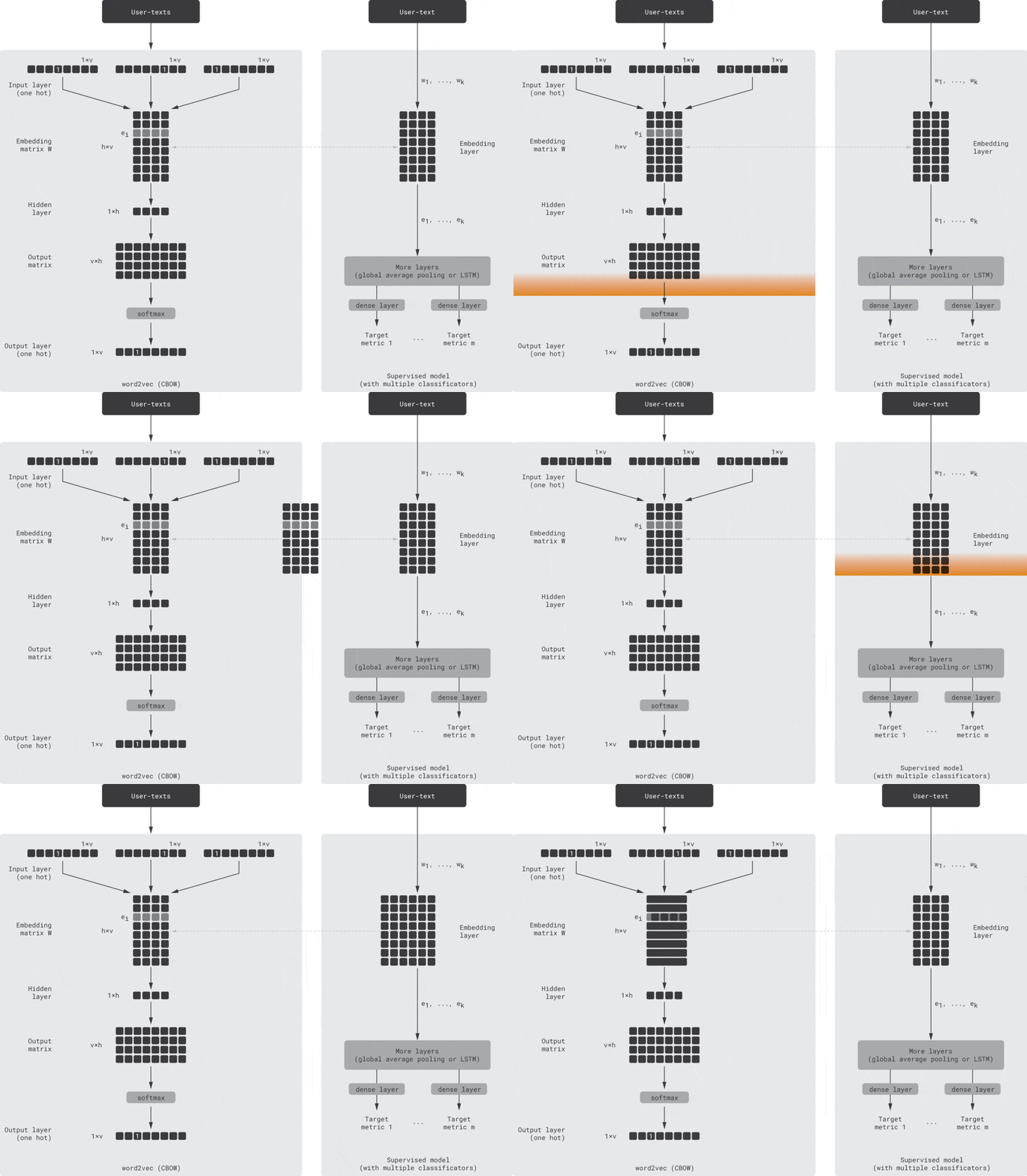
This guided learning helps to align the latent space with business metrics and improve the predictive power of embeddings.

Note that this approach has some similarities with the LSTM models we discussed in Step 1. In the case of guided word2vec, we start with an unsupervised method but enhance it with supervised guidance. In the case of LSTM, we start with a supervised model but extract embeddings from the hidden layer. Thus, both models can be viewed as hybrids. Moreover, one can use a multi-output LSTM model that predicts several metrics based on the same hidden layer [Zolna16], which makes the LSTM schema even more similar to the guided word2vec model described above.

Step 7: Learn with Autoencoders

In the NLP world, pioneering neural models with relatively simple architectures such as word2vec were gradually succeeded by more complex, deep, and specialized architectures, such as ELMo and BERT. Personalization and recommendation models follow a similar trajectory, and it is not uncommon to use more complex architectures than the vanilla LSTM and word2vec models we discussed previously. This can be illustrated with the autoencoder-based customer2vec model, which was evaluated as an alternative to word2vec-based models in several papers [Baldassini18, Seleznev18].

Conceptually, the architecture of autoencoder-based customer2vec is straightforward. The input of the model is aggregated fixed-length customer representation, which can be a vector of manual engineering features or a bag-of-words vector produced from a customer-text. This input is encoded into a low-dimensional representation using one or several neural layers, and then the original input is approximately reconstructed from this condensed representation. The network is trained to minimize the reconstruction error, and the low-dimensional representation is interpreted as a customer embedding. Optionally, the model can be extended with guiding metrics so that the overall loss function is a weighted sum of the reconstruction loss and guides losses, as shown below.

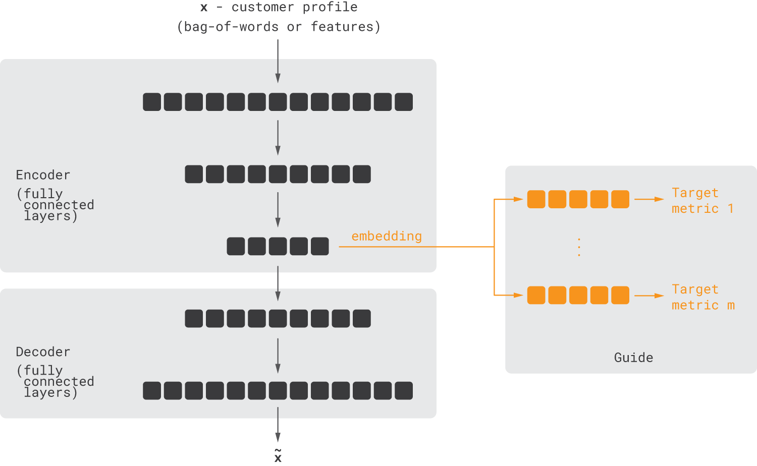
In practice, this approach may or may not provide advantages compared to word2vec, depending on the input data and use case, but in general, it is a competitive alternative.

Step 8: Incorporate Graph, Text, and Image Data

We have seen in the previous sections that customer2vec provides techniques for learning from behavioral, content, structured, and unstructured data. The last step is to explore this topic more thoroughly and better understand how various data types can be incorporated into product and customer embeddings.

Case Study 1: Financial Transactions

As a somewhat extreme example, let us consider a financial institution (e.g., a bank) that works with a large number of very different customers, including individuals, companies from different industries, public services, and so on. We assume that the institution observes transactions between these entities and can build a graph in which nodes represent entities and edges correspond to interactions. How can this graph be used to recommend financial services or perform entity segmentation?

The problem looks substantially more complex than what we discussed in the previous sections, but it can be quite naturally related to customer2vec formulation [Barbour20]. The main building block that enables this is node2vec, a generic algorithm for learning node embeddings in graphs [Grover16]. The basic idea of node2vec is relatively straightforward: multiple node sequences are generated by performing random walks across the graph, and then node embeddings are learned using vanilla word2vec, treating each node sequence as a sentence. A more formal description of this algorithm is presented below and is mostly self-explanatory.

Random walk subroutine
    Inputs and parameters:
        G = (V, E)       # input graph with nodes V and edges E
        U                # start node
        L                # max walk length
    random_walk(G, u):
        walk = [u]       # initialize walk
        c = u            # current node
        for i = 1 to L:
            neighbors = G.neighbors(c)
            c = sample(neighbors)        # sample the next node
            walk.append(c)
        return walk
Main node2vec routine
    Inputs and parameters:
        G = (V, E)       # input graph
        N                # walks per node 
    node2vec(G):
        walks = []
        for i = 1 to n:
            for u in V:
                walks.append(random_walk(G, u, L))
        return word2vec(walks)

The most complicated part of the node2vec algorithm is the sampling function, which chooses the node we move to from the current position. This function is designed as a stochastic process that balances breadth-first and depth-first searches. The breadth-first search tends to generate localized sequences that describe the structural role of the node (hubs, bridges, periphery, etc.), whereas the depth-first search produces sequences that describe how nodes are interconnected at a macro level. A balance between these two strategies is essential to produce good embeddings. However, we omit the details of the sampling process because they are immaterial to this conversation.

The node2vec algorithm provides the core functionality for learning embeddings from transaction graphs, social networks, and other similar data sources. The algorithm was designed as a domain-agnostic AutoML component that works well for a wide variety of tasks and graph topologies while requiring minimal tuning. The embedding produced by node2vec can be concatenated with embeddings produced by other customer2vec models and consumed by downstream processes. More advanced versions of this approach were used by Pinterest to build extreme-scale content recommendation systems [Eksombatchai17, Ying18].

Case Study 2: Video Recommendations

As a second example, let us discuss the video recommendation system created by YouTube [Covington16]. The models used in this system can be viewed as generalizations of collaborative filtering that incorporate additional behavior, content, and demographic data in a unified way.

The recommender has a two-part architecture: a candidate generation model that suggests hundreds of recommendation for each user and a ranking model that selects a few of the most relevant candidates. The models have similar architectures, but we focus on the candidate generation part to illustrate the approach and its relationship to customer2vec. The model is designed as a classification model that estimates the probability that user $u$ will watch video $i$ at time $t$, as follows:

$$
p(\text{watch video }i\text{ at time }t\ |\ u) = \frac{\exp(v_i\ u)}{\sum_{j\in V} \exp(v_i\ u)}
$$

where $V$ is the corpus of videos, $v_i$ is the embedding of the $i$-th video, and $u$ is the embedding of the user. Thus, learning user embeddings is at the core of the problem. This learning is done using the architecture shown in the figure below.

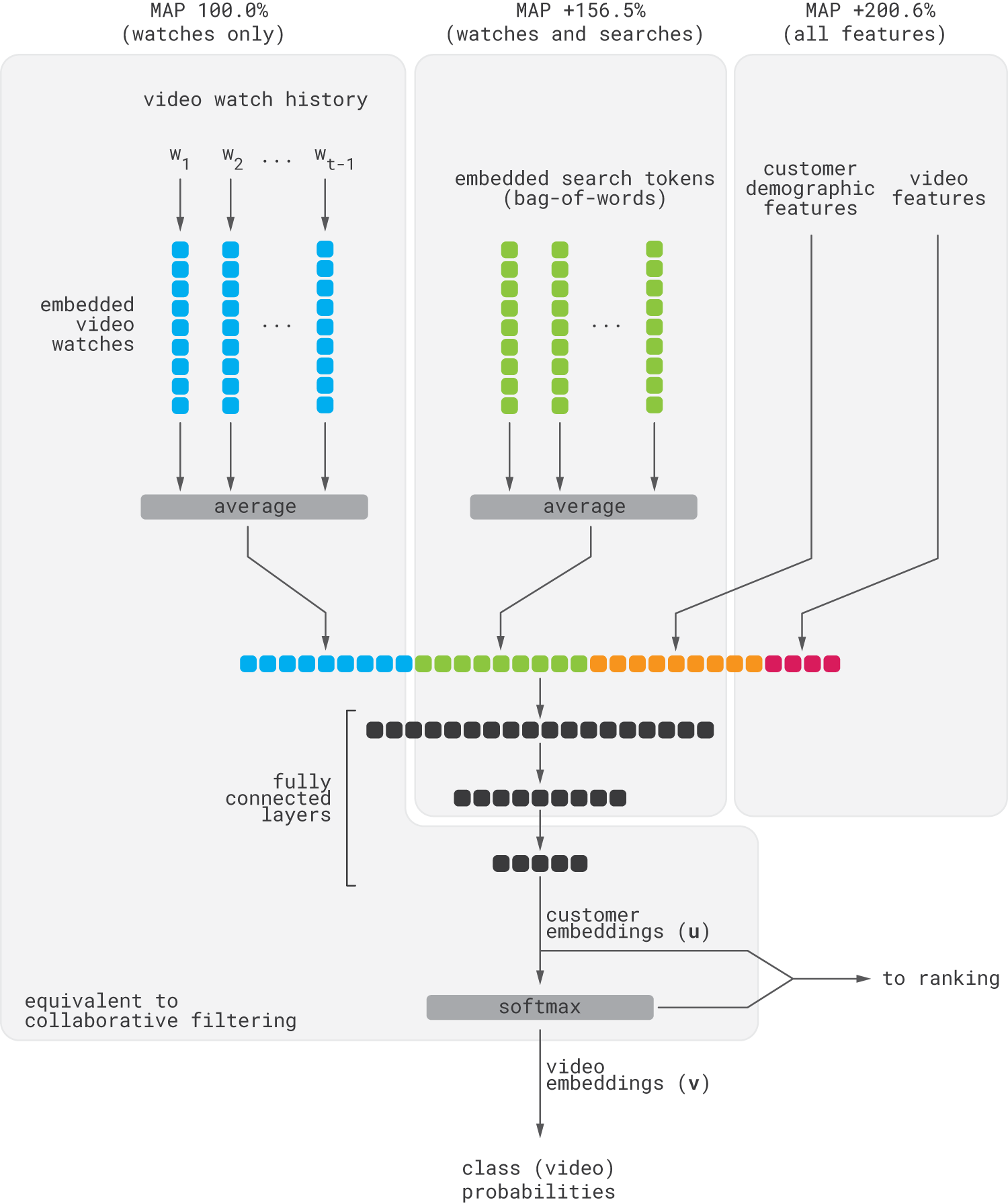
The network consumes several inputs. The first is the customer’s watch history. This is a sequence of sparse video IDs, each of which is mapped to dense embedding. Then, the embeddings are simply averaged into one fixed-length watch history embedding. The second input is the customer’s search history. Search queries are tokenized into unigrams and bigrams and then mapped to dense embeddings, which are averaged. Finally, demographic features and video metadata are added. The resulting vectors are concatenated and passed through a basic four-layer network to produce customer embeddings, $u$. Finally, customer embeddings are normalized into class probabilities (i.e., the probabilities of individual videos) using softmax, and vectors, $v_i$, are interpreted as video embeddings. Both customer and video embeddings are used in the downstream ranking processes.

Note that if one removes all inputs but watch history and all network layers but basic vector products, then the resulting network will be similar to traditional collaborative filtering with matrix factorization. The difference is that matrix factorization typically finds dense customer and product representations using algebraic procedures, and the truncated version of above network would find them through a stochastic gradient descent. The complete architecture can be viewed as a generalization of matrix factorization. According to the YouTube team, adding search embedding improves accuracy by about 50% compared to watch history only, and the complete set of features delivers close to 100% improvement.

Although the solution described above is much more complex than the basic models we discussed previously, it is fundamentally similar to guided customer2vec models, just like the LSTM-based models we discussed in Step 1. The guided learning paradigm enables us to seamlessly shift between supervised and unsupervised learning, depending on whether we want to focus on prediction (e.g., recommendations) or semantic analysis (e.g., clustering). In either case, we have a lot of flexibility for incorporating multiple heterogeneous inputs, including event sequences, texts, and images, as well as multiple target metrics due to the flexibility and expressiveness of neural networks.

Hands-on Tutorial

In the second part of this article, we implement the item2vec and customer2vec models and use them to analyze a public dataset containing a sample of over 3 million grocery orders from more than 200,000 Instacart users [Instacart2017]. We use the basic versions of the models described in the first part but spend a significant amount of time visualizing and analyzing the results.

Data Overview

We will use the following subset of files and fields, which are mostly self-explanatory:

products.csv
  | product_id | product_name                | aisle_id | department_id |
  | 1          | Chocolate Sandwich Cookies  | 61       | 19            |
  | 2          | All-Seasons Salt            | 104      | 13            |  
  | 3          | Robust Golden Oolong Tea    | 94       | 7             |  
  ...

departments.csv    # coarse categorization
  | department_id  | department |
  | 1              | frozen     |
  | 2              | other      |
  | 3              | bakery     |
  ...

aisles.csv         # fine-grained categorization
  | aisle_id  | aisle                 |
  | 1         | prepared soups salads | 
  | 2         | specialty cheeses     |
  | 3         | energy granola bars   |
  ...

order_products__prior.csv
  | order_id | product_id | add_to_cart_order * | ...  
  | 1        | 49302      | 1                   |  
  | 1        | 11109      | 2                   |  
  | 110246   | 3          | 0                   |
  ... 

orders.csv
  | order_id | user_id | ...
  | 2539329  | 1       |
  | 2398795  | 1       |  
  | 473747   | 1       |  
  ...

* in what order products were added to the cart

In total, we include 21 departments, 134 aisles, 206K users, 3.2M orders, and 32.4M order line items.

Building an Item2Vec Model Using Word2Vec

The first model we build is item2vec. We omit some parts of the implementation in the text below for the sake of clarity, but the complete code is provided in this notebook.

We start with data preparation. This is a very straightforward step because we just need to create a list of orders in which each order is a string of concatenated product IDs.

Data preparation for item2vec. Click to expand the code sample.

order_ds = orders_csv.merge(order_products_csv, 
                            left_on='order_id',
                            right_index=True)

# Creating sequences based on transactions
order_product_list = order_ds.sort_values(
                         ['user_id','order_id','add_to_cart_order'])
                         [['order_id','product_id']].values.tolist()

# Each entry of a corpus is one order represented by 
# a chronologically sorted sequence of product IDs.
product_corpus = []     
sentence = []
new_order_id = order_product_list[0][0]

for (order_id, product_id) in order_product_list:
    if new_order_id != order_id:
        product_corpus.append(sentence)
        sentence = []
        new_order_id = order_id
    sentence.append(str(product_id))

The second step is model training. We use the word2vec implementation provided by the gensim library and feed the corpus or order-texts into it.

from gensim.models import Word2Vec
import multiprocessing as mp

WORD_DIM = 200   # dimensionality of the embedding space
model = Word2Vec(product_corpus, 
                 window=5, 
                 size=WORD_DIM, 
                 workers=mp.cpu_count() - 2, 
                 min_count=100)

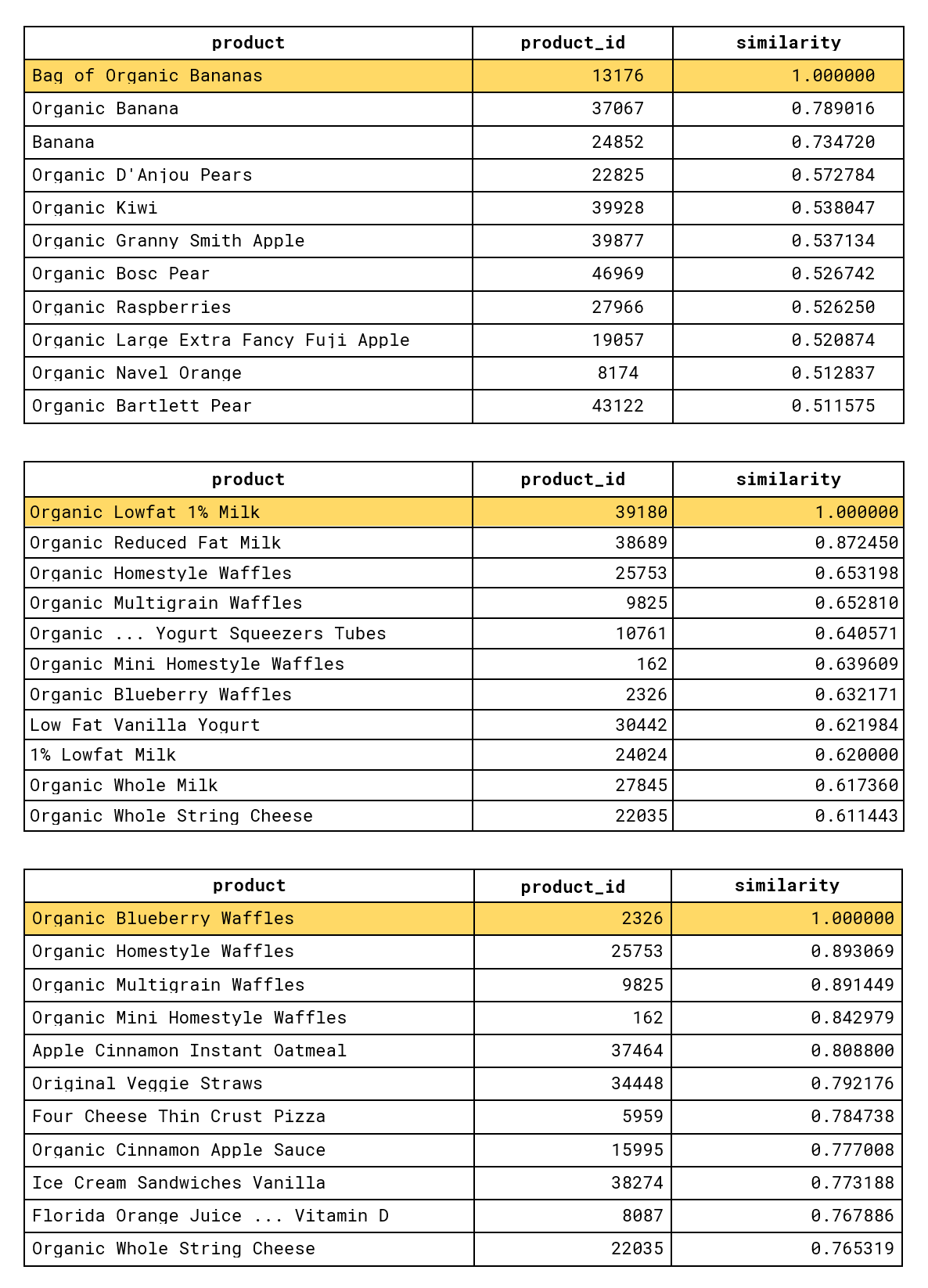
The next step is to explore and analyze the embedding space produced by the model. First, let us do a quick reality check and examine the neighborhoods around several common products to make sure that the embeddings look reasonable. We can easily do this using a model API that allows us to fetch the nearest neighbors (in terms of embedding distances) for a given token.

Exploring nearest neighbors for several products. Click to expand the code sample.

def to_product_name(id, columns='product_name'):
    Return products_csv[products_csv.product_id==id][columns].values.tolist()[0]

def most_similar_readable(model, product_id, topn=10):
    similar_list = [(product_id, 1.0)] + model.wv.most_similar(str(product_id), 
                                                               topn=topn)
    return pd.DataFrame([( to_product_name(int(id)), int(id), similarity ) for 
                         (id, similarity) in similar_list],
                        columns=['product', 'product_id', 'similarity'])

for product_id in [13176, # Bag of Organic Bananas 
                   39180, # Organic Lowfat 1% Milk
                   2326]: # Organic Blueberry Waffles
    most_similar_readable(model, product_id)

This produces results that align with the common product categorization: there are clusters of fruits, dairy products, and desserts.

Next, let us visualize the structure and geometry of the semantic space using a two-dimensional t-SNE projection. We color the products in the projection according to their department labels to understand how well the embeddings are aligned with the ground truth semantics.

Visualizing the semantic space using t-SNE. Click to expand the code sample.

from sklearn.manifold import TSNE
from sklearn.metrics import pairwise_distances

# prepare inputs for t-SNE
word_vectors = model.wv
vocab = list(model.wv.vocab.keys())
item2vector_dict = {arg:model.wv[arg] for arg in vocab}
X = pd.DataFrame(item2vector_dict).T.values

# perform t-SNE
distance_matrix = pairwise_distances(X, X, metric='cosine', n_jobs=-1)
tsne = TSNE(metric="precomputed", n_components=2, 
            verbose=1, perplexity=30, n_iter=500)
tsne_results = tsne.fit_transform(distance_matrix)

# prepare t-SNE outputs for visualization
df_semantic_item = pd.DataFrame({'product_id': vocab})
df_semantic_item['tsne-2d-one'] = tsne_results[:,0]
df_semantic_item['tsne-2d-two'] = tsne_results[:,1]
df_semantic_item['product_id'] = df_semantic_item['product_id'].astype(int)

# join the embeddings with department and aisle names
df_semantic_item = df_semantic_item.merge(data_dict['products'], 
                                          on='product_id', how='left')
df_semantic_item = df_semantic_item.merge(data_dict['aisles'],
                                          on='aisle_id', how='left')
df_semantic_item = df_semantic_item.merge(data_dict['departments'], 
                                          on='department_id', how='left')

# visualize the semantic space and its mapping to the departments
sns.scatterplot(
    x="tsne-2d-one", y="tsne-2d-two",
    hue='department',
    palette=sns.color_palette("hls", n_department),
    data=df_semantic_item,
    legend="full",
    alpha=0.3
)

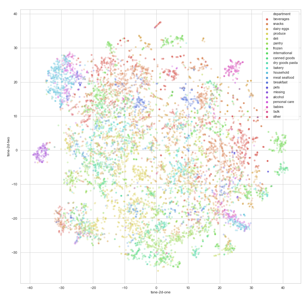
We can see that the latent space has a reasonably good structure that is generally aligned with department labels. By performing the same visualization for aisles (which have a more granular categorization than departments), we can observe a similar degree of alignment. Note, however, that we do not aim to exactly reproduce the department or aisle clusters; rather, our goal is to create embeddings that describe behavioral and semantic patterns, which do not necessarily match static labels.

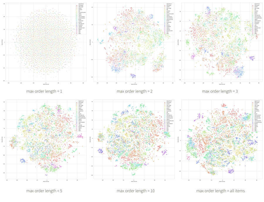
It is also useful to visualize how the embedding space shapes up as one increases the length of order-texts (sentences). In the figure below, we create the upper-left plot by training our model on order-texts truncated to the first product ID. Then, we increase the length to two products, and so on. As expected, the first space is non-informative because there are no product co-occurrences to learn from, but the manifold takes shape very quickly.

Finally, let us examine the relationship between this t-SNE projection and the original 200-dimensional space. We can do a quick check using silhouette coefficients. Recall that the silhouette coefficient for a set of clustered points is defined as follows:

• First, we compute the mean intra-cluster distance ($a$) and the mean nearest-cluster distance ($b$) for each point.
• Second, we compute the silhouette coefficient for each point as $(b - a) / max(a, b)$. This basically characterizes how well a point’s own cluster is separated from surrounding clusters.
• Finally, the silhouette coefficient for the entire set is simply the average of the points’ coefficients.

The coefficient of $-1.0$ is the worst value (poor separation), and the coefficient of $+1.0$ is the best value. We can straightforwardly calculate the silhouette coefficients for the department pseudo-clusters visualized above for both the original space and the t-SNE projection using scikit-learn.

Silhouette scores for department pseudo-clusters. Click to expand the code sample.

from sklearn.metrics import silhouette_samples, silhouette_score

for space_name, space in {'t-SNE': tsne_results, 
                          'original': model.wv.vectors}.items():
    for entity in ['department', 'aisle']:
        s = silhouette_score(space, df_semantic_item[entity], metric="cosine")
        print(f"Score on {space_name} space for {entity}s is {s:.4}")

--------------

#> Score on t-SNE space for departments is -0.4912
#> Score on t-SNE space for aisles is -0.7124
#> Score on original space for departments is -0.05162
#> Score on original space for aisles is : -0.1148

As shown, the separation in the complete space is significantly better than in the projection, but again, we do not aim to perfectly align with the nominal categorization. We continue to explore the relationship between the nominal categories and behavioral clusters in the latent embedding space in the next section.

Building a Customer2Vec Model Using Doc2Vec

In this section, we discuss the development of the customer2vec model. As discussed in the first part of the article, customer2vec techniques can be approached from several different angles, including customer scoring, recommendations, and segmentation. In this section, we choose to focus on segmentation. We skip some parts of the implementation for the sake of brevity, but the complete source code is available in this notebook.

The first step is to establish a baseline using traditional clustering in a space of hand-crafted features. We take a sample of 50,000 users and represent each user as a vector of relative purchase frequencies in each department and aisle as follows (155 features in total):

Next, we perform a t-SNE projection of this hand-crafted feature space and visualize it in the scatterplot below (in which each point is a customer).

t-SNE of hand-crafted customer features. Click to expand the code sample.

from sklearn.preprocessing import MinMaxScaler
mm_scale = MinMaxScaler()

# feature_df is the dataframe with customer features
feature_df_scale = pd.DataFrame(mm_scale.fit_transform(feature_df),
                                columns=feature_df.columns,
                                index=feature_df.index.values)

tsne_doc_features = TSNE(n_components=2, verbose=1, perplexity=30, n_iter=500)
tsne_features_doc = tsne_doc_features.fit_transform(feature_df_scale.values)

tsne_doc_features = pd.DataFrame({'user_id':feature_df.index.values})
tsne_doc_features['tsne-2d-one'] = tsne_features_doc[:,0]
tsne_doc_features['tsne-2d-two'] = tsne_features_doc[:,1]

plt.figure(figsize=(16, 10))
sns.scatterplot(
    x="tsne-2d-one", y="tsne-2d-two",
    data=tsne_doc_features,
    legend="full",
    alpha=0.3
)

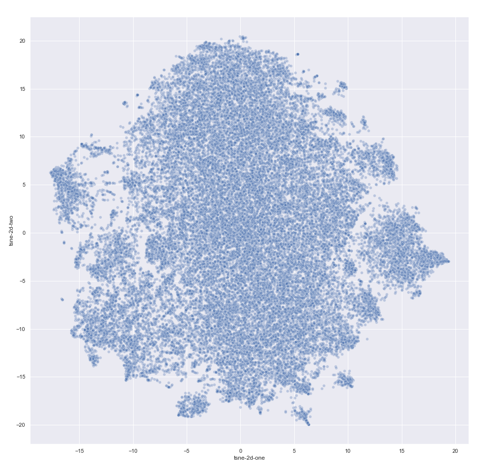
We can see from the t-SNE visualization that it is possible to separate 2–3 clusters, but this feature space is not a good choice for customer segmentation. If we go along this route, we have to develop more advanced features and incorporate more domain knowledge to obtain meaningful clusters.

For the customer2vec model, we simply combine all product IDs from past customer orders in chronological order into strings:

Data preparation for customer2vec. Click to expand the code sample.

orders.sort_values(by=['user_id','order_number','add_to_cart_order'], 
                   inplace=True)

orders_by_uid = orders.groupby("user_id")
                      .apply(lambda order: ' '.join(order['product_id'].tolist()))

orders_by_uid = pd.DataFrame(orders_by_uid,  
                             columns=['all_orders'])
orders_by_uid.reset_index(inplace=True)
orders_by_uid.user_id = orders_by_uid.user_id.astype(str)

Next, we train the doc2vec model based on this input. This step is relatively straightforward; the only customization we perform is manual annealing of the learning rate.

Customer2vec model training. Click to expand the code sample.

from gensim.models.doc2vec import TaggedDocument

EMBEDDING_DIM = 200    # dimensionality of user representation

class TaggedDocumentIterator(object):
    def __iter__(self):
        for row in self.df.itertuples():
            yield TaggedDocument(
                     words=dict(row._asdict())['all_orders'].split(),
                     tags=[dict(row._asdict())['user_id']])

it = TaggedDocumentIterator(orders_by_uid)

doc_model = gensim.models.Doc2Vec(vector_size=EMBEDDING_DIM, 
                                  window=5, 
                                  min_count=10, 
                                  workers=mp.cpu_count(),
                                  alpha=0.055, 
                                  min_alpha=0.055,
                                  epochs=120)

train_corpus = list(it)

doc_model.build_vocab(train_corpus)

for epoch in range(10):
    doc_model.alpha -= 0.005                    # decrease the learning rate
    doc_model.min_alpha = doc_model.alpha       
    doc_model.train(train_corpus, 
                    total_examples=doc_model.corpus_count, 
                    epochs=doc_model.iter)

Next, we sample the same users as for the baseline and project their embedding using t-SNE:

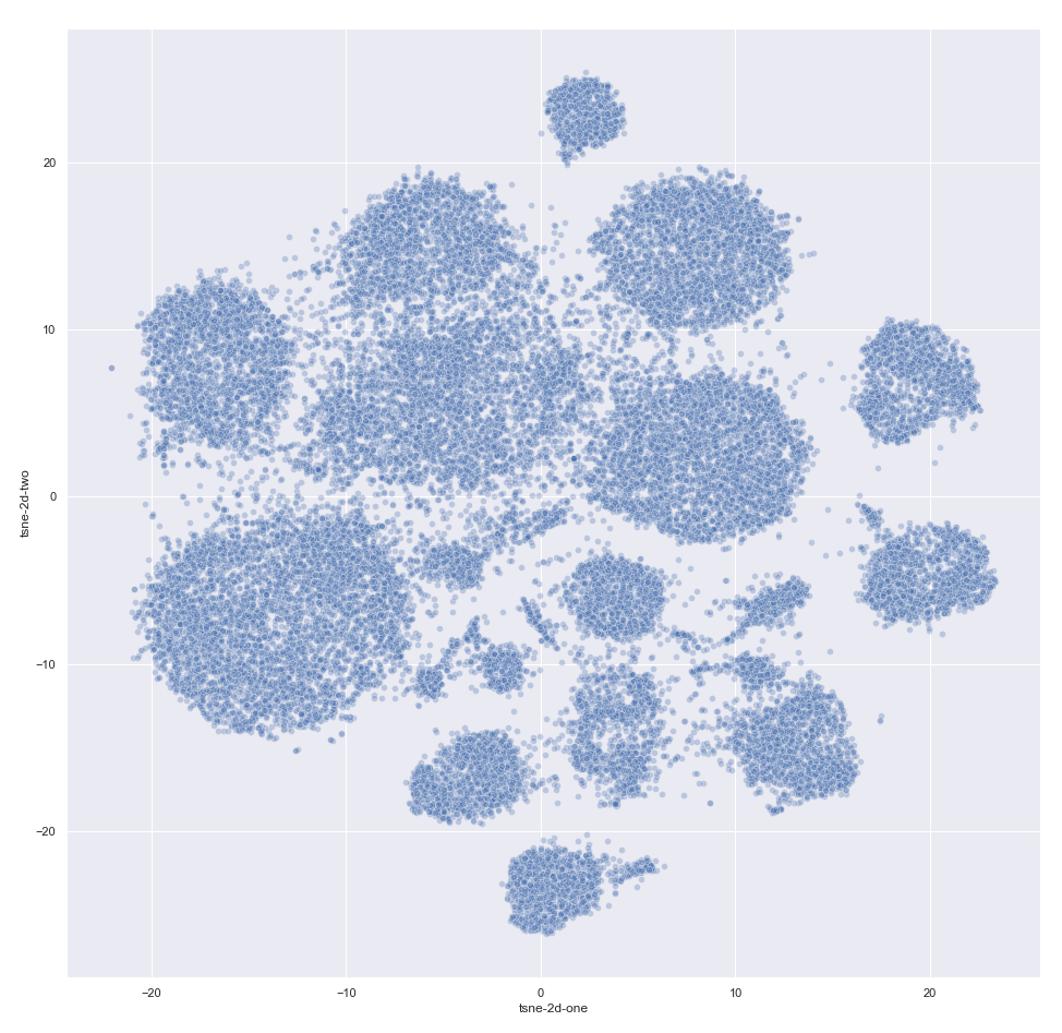
This result seems to be much better than our baseline attempt. We run k-means on this sample for a different number of clusters and determine that a total of 12 clusters is optimal in terms of the silhouette score.

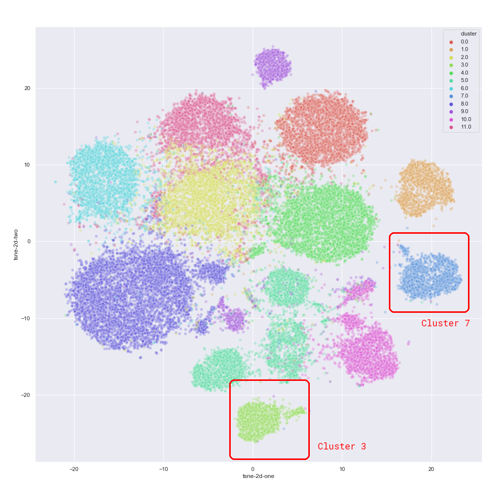
The last step is to analyze the semantics of these clusters. We have already seen that clusters produced by the item2vec model are aligned with the department labels, so we can start by computing the average purchase frequencies in each department for each cluster.

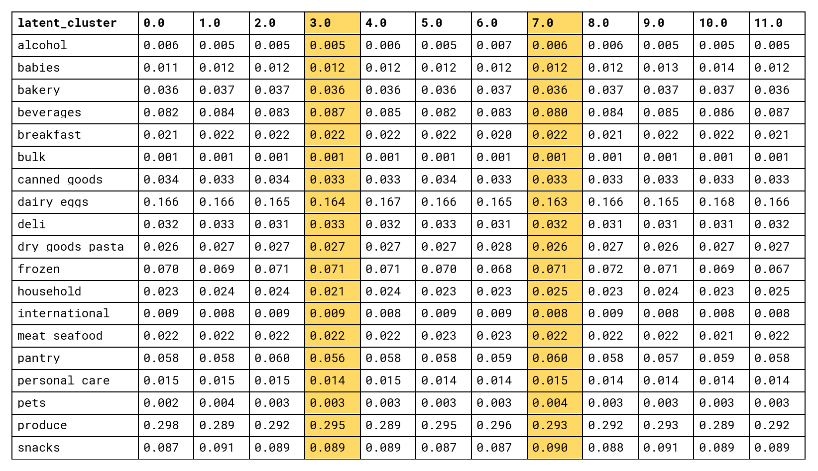
Unfortunately, this does not work well; although embedding clusters are separated quite well, their basic department statistics are almost identical (we chose to highlight clusters #3 and #7 in the plot and in the table as illustrative examples). This was expected because our baseline attempt at segmentation in the space of similar features did not work either.

Let us now examine individual samples from the clusters to see if there are any patterns. To do this, we sample several customers from clusters #3 and #7 and replace product IDs in customer-texts with human-readable product names:

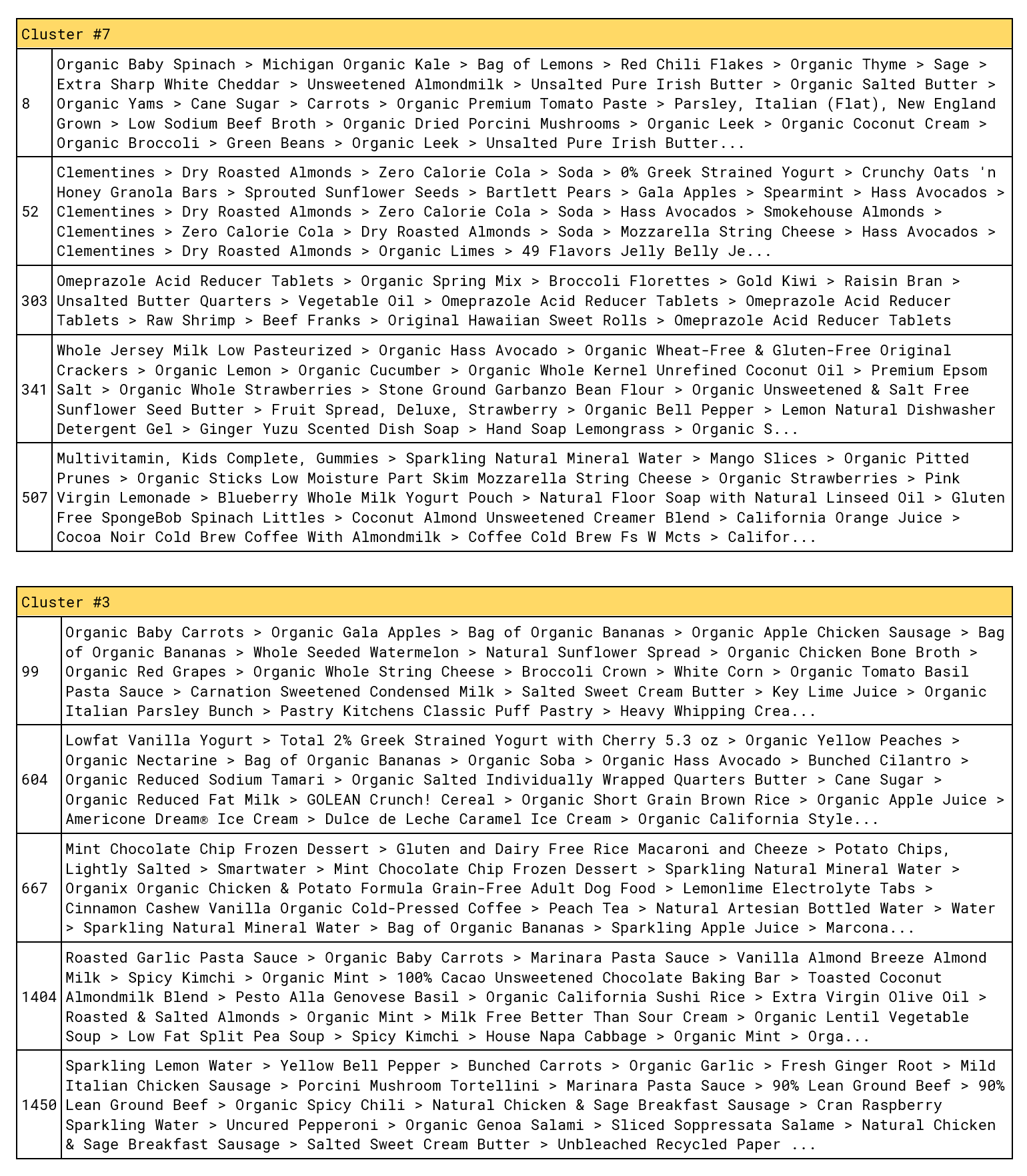
This result makes more sense; cluster 7 is dominated by healthy low-calorie products (vegetables, nonfat dairy, vitamins, etc.), whereas cluster 3 has a significant presence of high-calorie products (sausage, rice, bananas, frozen desserts, ice cream, pasta sauce, etc.). This fine structure, however, is not clearly visible in the aggregated department-level metrics.

Conclusions

We have seen that NLP-style models are powerful building blocks for customer intelligence and personalization applications. These models are conceptually simple and easy to implement using standard components like word2vec. They also have minimal data engineering requirements and, more importantly, can learn directly from server logs or provide AutoML functionality for downstream models. Finally, these models generally outperform traditional methods in terms of predictive power and the quality of semantic analysis due to their specialization in sequence modeling.

In this article, we mainly focused on unsupervised representation learning, AutoML, and semantic analysis capabilities of neural models in the context of customer intelligence. We discussed their applicability to predictive modeling use cases but did not explore this topic extensively. However, readers should keep in mind that customer2vec methods are related to deep learning based recommender systems, which are the focus of another large stream of research and industrial developments. The benefits offered by deep learning recommenders are similar to those of customer2vec: explicit modeling of event sequences, seamless fusion of behavior and context data, and incorporation of multiple data types, including texts, images, and graphs. One of the best-known examples of such a solution is YouTube’s deep learning based video recommender [Covington16]. Systematic discussions of this topic can be found in [Zhang19] and other overviews.

Finally, let us note that although customer2vec and other neural personalization models borrow many ideas from NLP and computer vision, they significantly lag behind in terms of sophistication, which indicates that there is a lot of room for improvement. Some ideas that were very successful in the area of NLP, such as transfer learning and transformers, have not yet been adequately adopted in the area of customer analytics.

References

1. [ Microsoft ] Barkan O., Koenigstein N. -- Item2Vec: Neural Item Embedding for Collaborative Filtering
2. [ Myntra ] Arora S., Warrier D. -- Decoding Fashion Contexts Using Word Embeddings, 2016
3. [ Rakuten ] Phi V., Chen L., Hirate Y. -- Distributed Representation-based Recommender Systems in E-commerce, 2016
4. [ RTB House ] Zolna K., Bartlomiej R. -- User2vec: User Modeling Using LSTM Networks, 2016
5. [ MediaGamma ] Stiebellehner S., Wang J., Yuan S. -- Learning Continuous User Representations Through Hybrid Filtering with doc2vec, 2017
6. [ Yandex ] Seleznev N., Irkhin I., Kantor V. -- Automated Extraction of Rider’s Attributes Based on Taxi Mobile Application Activity Logs, 2018
7. [ BBVA ] Baldassini L., Serrano J. -- client2vec: Towards Systematic Baselines for Banking Applications, 2018
8. [ Zalando ] Lang T., Rettenmeier M. -- Understanding Consumer Behavior with Recurrent Neural Networks, 2017
9. [ Netflix ] Koren Y., Bell R., Volinsky C. -- Matrix Factorization Techniques for Recommender Systems, 2009
10. [ Snap Inc. ] Yang C., Shi X., Luo J., Han J. -- I Know You'll Be Back: Interpretable New User Clustering and Churn Prediction on a Mobile Social Application, 2018
11. [ Netflix ] Hidasi B., Karatzoglou A., Baltrunas L., Tikk D. -- Session-based Recommendations with Recurrent Neural Networks, 2016
12. Grover A., Leskovec J. -- node2vec: Scalable Feature Learning for Networks, 2016
13. [ Q2ebanking ] Barbour J. -- Learning Node Embedding in Transaction Networks, 2020
14. [ Pinterest ] Ying R., He R., Chen K., Eksombatchai P., Hamilton W., Leskovec J. -- Graph Convolutional Neural Networks for Web-Scale Recommender Systems, 2018
15. [ Pinterest ] Eksombatchai C., Jindal P., Liu J., Liu Y., Sharma R., Sugnet C., Ulrich M., Leskovec J. -- Pixie: A System for Recommending 3+ Billion Items to 200+ Million Users in Real-Time, 2017
16. [ Google / YouTube ] Covington P., Adams J., Sargin E. -- Deep Neural Networks for YouTube Recommendations, 2016
17. Zhang S., Yao L., Sun A., Tay Y. -- Deep Learning based Recommender System: A Survey and New Perspectives, 2019
18. [ Instacart ] The Instacart Online Grocery Shopping Dataset 2017, Accessed from https://www.instacart.com/datasets/grocery-shopping-2017