Deep reinforcement learning for supply chain and price optimization

Supply chain and price management were among the first areas of enterprise operations that adopted data science and combinatorial optimization methods and have a long history of using these techniques with great success. Although a wide range of traditional optimization methods are available for inventory and price management applications, deep reinforcement learning pricing has the potential to substantially improve the optimization capabilities for these and other types of enterprise operations due to impressive recent advances in the development of generic self-learning algorithms for optimal control. In this article, we explore how deep reinforcement learning methods can be applied in several basic supply chain and price management scenarios.
This article is structured as a hands-on tutorial that describes how to develop, debug, and evaluate reinforcement learning optimizers using PyTorch and RLlib:

• We start with a simple motivating example that illustrates how slight modifications of traditional price optimization problems can result in complex behavior and increase optimization complexity.
• Next, we use this simplistic price management environment to develop and evaluate our first optimizer using only a vanilla PyTorch toolkit.
• We then discuss how the implementation can be drastically simplified and made more robust with RLlib, an open-source library for reinforcement learning.
• Next, we develop a more complex supply chain environment that includes a factory, several warehouses, and transportation. For this environment, we first implement a baseline solution using a traditional inventory management policy. Then we show how this baseline can be improved using continuous control algorithms provided by RLlib.
• Finally, we conclude the article with a discussion of how deep reinforcement learning algorithms and platforms can be applied in practical enterprise settings.
  
  

Introductory example: Differential price response and Hi-Lo pricing

The traditional price optimization process in retail or manufacturing environments is typically framed as a what-if analysis of different pricing scenarios using some sort of demand model. In many cases, the development of a demand model is challenging because it has to properly capture a wide range of factors and variables that influence demand, including regular prices, discounts, marketing activities, seasonality, competitor prices, cross-product cannibalization, and halo effects. Once the demand model is developed, however, the optimization process for pricing decisions is relatively straightforward, and standard techniques such as linear or integer programming typically suffice. For instance, consider an apparel retailer that purchases a seasonal product at the beginning of the season and has to sell it out by the end of the period. Assuming that a retailer chooses pricing levels from a discrete set (e.g., \$59.90, \$69.90, etc.) and can make price changes frequently (e.g., weekly), we can pose the following optimization problem:

$$
\begin{aligned}
\max \ \ & \sum_t \sum_j p_j \cdot d(t, j) \cdot x_{tj} \\
\text{subject to} \ \ & \sum_j x_{tj} = 1, \quad \text{for all } t \\
&\sum_t \sum_j d(t, j) \cdot x_{tj} = c \\
&x_{tj} \in {0,1}
\end{aligned}
$$

where $t$ iterates over time intervals, $j$ is an index that iterates over the valid price levels, $p_j$ is the price with index $j$, $d(t, j)$ is the demand at time $t$ given price level $j$, $c$ is the inventory level at the beginning of the season, and $x_{tj}$ is a binary dummy variable that is equal to one if price $j$ is assigned to time interval $t$, and zero otherwise. The first constraint ensures that each time interval has only one price, and the second constraint ensures that all demands sum up to the available stock level. This is an integer programming problem that can be solved using conventional optimization libraries.

The above model is quite flexible because it allows for a price-demand function of an arbitrary shape (linear, constant elasticity, etc.) and arbitrary seasonal patterns. It can also be straightforwardly extended to support joint price optimization for multiple products. The model, however, assumes no dependency between time intervals.

Let us now explore how the dependencies between time intervals can impact the optimization process. In the real world, demand depends not only on the absolute price level but can also be impacted by the magnitude of recent price changes—price decrease can create a temporary demand splash, while price increase can result in a temporary demand drop. The impact of price changes can also be asymmetric, so that price increases have a much bigger or smaller impact than the decreases. We can codify these assumptions using the following price-demand function:

$$
\begin{aligned}
d(p_t, p_{t-1}) &= d_0 - k\cdot p_t - a\cdot s( (p_t - p_{t-1})^+) + b\cdot s( (p_t - p_{t-1})^-) \\
&\\
\text{where}\\
&\\
x^+ &= x\text{ if } x>0 \text{, and } 0 \text{ otherwise} \\
x^- &= x\text{ if } x<0 \text{, and } 0 \text{ otherwise} \\
\end{aligned}
$$

and $p_t$ is the price for the current time interval and $p_{t-1}$ is the price for the previous time interval. The first two terms correspond to a linear demand model with intercept $d_0$ and slope $k$. The second two terms model the response on a price change between two intervals. Coefficients $a$ and $b$ define the sensitivity to positive and negative price changes, respectively, and $s$ is a shock function that can be used to specify a non-linear dependency between the price change and demand. For the sake of illustration, we assume that $s(x) = \sqrt x$.

Let us now investigate what the optimal price schedule for such a price-response function looks like. We start by implementing functions that compute profit for a given price schedule (a vector of prices for several time steps):

Price optimization environment. Click to expand the code sample.

## Environment simulator
def plus(x):
    return 0 if x < 0 else x

def minus(x):
    return 0 if x > 0 else -x

def shock(x):
    return np.sqrt(x)

# Demand at time step t for current price p_t and previous price p_t_1
def q_t(p_t, p_t_1, q_0, k, a, b):
  return plus(q_0 - k*p_t - a*shock(plus(p_t - p_t_1)) + b*shock(minus(p_t - p_t_1)))

# Profit at time step t
def profit_t(p_t, p_t_1, q_0, k, a, b, unit_cost):
  return q_t(p_t, p_t_1, q_0, k, a, b)*(p_t - unit_cost) 

# Total profit for price vector p over len(p) time steps
def profit_total(p, unit_cost, q_0, k, a, b):
  return profit_t(p[0], p[0], q_0, k, 0, 0, unit_cost) + 
         sum(map(lambda t: profit_t(p[t], p[t-1], q_0, k, a, b, unit_cost), range(len(p))))

## Environment parameters
T = 20                # Time steps in the price schedule
price_max = 500       # Maximum valid price, dollars
price_step = 10       # Minimum valid price change, dollars
q_0 = 5000            # Intercept in the demand function q_t
k = 20                # Slope in the demand function, q_t
unit_cost = 100       # Product production cost, dollars
a_q = 300             # Response coefficient for price increase 
b_q = 100             # Response coefficient for price decrease

## Partial bindings for readability
def profit_t_response(p_t, p_t_1):
  return profit_t(p_t, p_t_1, q_0, k, a_q, b_q, unit_cost)

def profit_response(p):
  return profit_total(p, unit_cost, q_0, k, a_q, b_q)

We can visualize this environment by plotting profit functions that correspond to different magnitudes of price changes (see the complete notebook for implementation details):

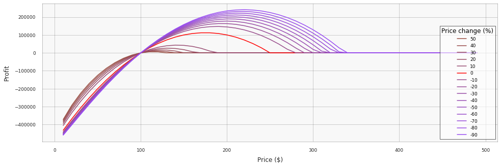
We can see that price increases "deflate" the baseline profit function, while price decreases "inflate" it. Next, we obtain our first profit baseline by searching for the optimal single (constant) price:

Price optimization: Constant price. Click to expand the code sample.

profits = np.array([ profit_response(np.repeat(p, T)) for p in price_grid ])
p_idx = np.argmax(profits)                 # index of the profit-maximizing price
price_opt_const = price_grid[p_idx]        # profit-maximizing price
print(f'Optimal price is {price_opt_const}, achieved profit is {profits[p_idx]}')

#> Optimal price is 170, achieved profit is 2352000.0

The constant-price schedule is not optimal for this environment, and we can improve profits through greedy optimization: start with finding the optimal price for the first time step, then optimize the second time step having frozen the first one, and so on:

Price optimization: Dynamic price. Click to expand the code sample.

def find_optimal_price_t(p_baseline, price_grid, t):   # evalutes all possible price schedules 
  p_grid = np.tile(p_baseline, (len(price_grid), 1))   # derived from the baseline by  
  p_grid[:, t] = price_grid                            # changing the price at time t
  profit_grid = np.array([ profit_response(p) for p in p_grid ])
  return price_grid[ np.argmax(profit_grid) ]

p_opt = np.repeat(price_opt_const, T)                  # start with the constant price schedule
for t in range(T):                                     # and optimize one price at a time
  price_t = find_optimal_price_t(p_opt, price_grid, t)
  p_opt[t] = price_t

print(f'Achieved profit is {profit_response(p_opt)}')
plt.plot(range(len(p_opt)), p_opt, c='red')

#> Achieved profit is 2903637.2

This approach improves profit significantly and produces the following price schedule:

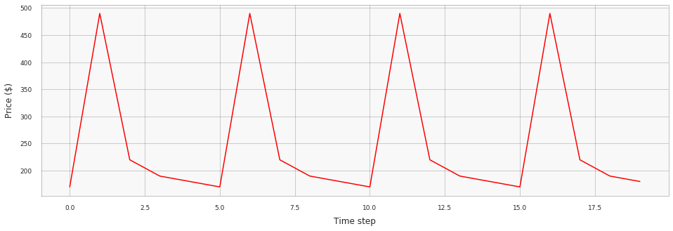
This result is remarkable: a simple temporal dependency inside the price-demand function dictates a complex pricing strategy with price surges and discounts. It can be viewed as a formal justification of the Hi-Lo pricing strategy used by many retailers; we see how altering regular and promotional prices helps to maximize profit.

The above example sheds light on the relationship between price management and reinforcement learning optimization. The price-response function we have defined is essentially a differential equation where the profit depends not only on the current price action but also on the dynamics of the price. It is expected that such equations can exhibit very complicated behavior, especially over long-time intervals, so the corresponding control policies can also become complicated. Optimization of such policies thus requires powerful and flexible methods, such as deep reinforcement learning. We explore this approach in the following sections.

Case study 1: Pricing policy optimization using DQN

Although the greedy algorithm we implemented above produces the optimal pricing schedule for a simple differential price-response function, it becomes increasingly more challenging to reduce the problem to standard formulations, such as linear or integer programming, as we add more constraints or interdependencies. In this section, we approach the problem from a different perspective and apply a generic Deep Q Network (DQN) algorithm to learn the optimal price control policy.

We use the original DQN in this example because it is a reasonably simple starting point that illustrates the main concepts of modern reinforcement learning. In practical settings, one is likely to use either more recent modifications of the original DQN or alternative algorithms—we will discuss this topic more thoroughly at the end of the article.

Although DQN implementations are available in most reinforcement learning libraries, we chose to implement the basic version of DQN from scratch to provide a clearer picture of how DQN is applied to this particular environment and to demonstrate several debugging techniques. Readers who are familiar with DQN can skip the next two sections that describe the core algorithm and its PyTorch implementation.

Defining the environment

Reinforcement learning considers the setup where an agent interacts with the environment in discrete time steps with the goal of learning a reward-maximizing behavior policy. At each time step $t$, with a given state $s$, the agent takes an action $a$ according to its policy $\pi(s) \rightarrow a$ and receives the reward $r$ moving to the next state $s’$. We redefine our pricing environment in these reinforcement learning terms as follows.

First, we encode the state of the environment at any time step $t$ as a vector of prices for all previous time steps concatenated with one-hot encoding of the time step itself:

$$
s_t = \left( p_{t-1}, p_{t-2}, \ldots, p_{0}, 0, \ldots \right)\ |\ \left(0, \ldots, 1, \ldots, 0 \right)
$$

Next, the action $a$ for every time step is just an index in the array of valid price levels. Finally, the reward $r$ is simply the profit of the seller. Our goal is to find a policy that prescribes a pricing action based on the current state in a way that the total profit for a selling season (episode) is maximized.

Overview of the DQN algorithm

In this section, we briefly review the original DQN algorithm ^[1]. The goal of the algorithm is to learn an action policy $\pi$ that maximizes the total discounted cumulative reward (also known as the return) earned during the episode of $T$ time steps:

$$
R = \sum_{t=0}^T \gamma^t r_t
$$

Such a policy can be defined if we know a function that estimates the expected return based on the current state and next action, under the assumption that all subsequent actions will also be taken according to the policy:

$$
Q^{\pi}(s,a) = \mathbb{E}_{s,a}\left[R\right]
$$

Assuming that this function (known as the Q-function) is known, the policy can be straightforwardly defined as follows to maximize the return:

$$
\pi(s) = \underset{a}{\text{argmax}}\ Q(s,a)
$$

We can combine the above definitions into the following recursive equation (the Bellman equation):

$$
Q^{\pi}(s,a) = r + \gamma\max_{a'} Q(s', a')
$$

where $s'$ and $a'$ are the next state and the action taken in that state, respectively. If we estimate the Q-function using some approximator, then the quality of the approximation can be measured using the difference between the two sides of this equation:

$$
\delta = Q^{\pi}(s,a) - \left( r +\gamma\max_{a'} Q(s', a') \right)
$$

This value is called the temporal difference error. The main idea behind DQN is to train a deep neural network to approximate the Q-function using the temporal difference error as the loss function. In principle, the training process can be straightforward:

1. Initialize the network. Its input corresponds to state representation, while output is a vector of Q-values for all actions.
2. For each time step:
   1. Estimate Q-values using the network.
   2. Execute the action with the maximum Q-value and observe the reward.
   3. Calculate the temporal difference error.
   4. Update the network's parameters using stochastic gradient descent. The loss function is derived from the temporal difference error.

This simple approach, however, is known to be unstable for training complex non-linear approximators, such as deep neural networks. DQN addresses this issue using two techniques:

• Replay buffer. One of the problems with the basic training process described above is that sequential observations are usually correlated, while network training generally requires independently distributed samples. DQN works around this by accumulating multiple observed transitions $(s,a,r,s’)$ in a buffer and sampling batches of such transitions to retrain the network. The buffer is typically chosen large enough to minimize correlations between samples.
• Target networks. The second problem with the basic process is that network parameters are updated based on the loss function computed using Q-values produced by the same network. In other words, the learning target moves simultaneously with the parameters we are trying to learn, making the optimization process unstable. DQN mitigates this issue by maintaining two instances of the network. The first one is used to take actions and is continuously updated as described above. The second one, called a target network, is a lagged copy of the first one and used specifically to calculate Q-values for the loss function (i.e., target). This technique helps to stabilize the learning process.

Combining the basic learning process with these two ideas, we obtain the DQN algorithm:

The last concern that we need to address is how the action is chosen based on Q-values estimated by the network. A policy that always takes action with the maximum Q-value will not work well because the learning process will not sufficiently explore the environment, so we choose to randomize the action selection process. More specifically, we use $\varepsilon$-greedy policy that takes the action with the maximum Q-value with the probability of $1-\varepsilon$ and a random action with the probability of $\varepsilon$. We also use the annealing technique starting with a relatively large value of $\varepsilon$ and gradually decreasing it from one training episode to another.

More details about DQN can be found in the original paper ^[1:1]; its modifications and extensions are summarized in ^[2], and more thorough treatments of Q-learning are provided in excellent books by Sutton and Barto ^[3], Graesser and Keng ^[4].

Implementing DQN using PyTorch

Our next step is to implement the DQN algorithm using PyTorch ^[5]. We develop all major components in this section, and the complete implementation with all auxiliary functions is available in this notebook.

The first step is to implement a memory buffer that will be used to accumulate observed transitions and replay them during the network training. The implementation is straightforward, as it is just a generic cyclic buffer:

Experience replay buffer. Click to expand the code sample.

Transition = namedtuple('Transition', ('state', 'action', 'next_state', 'reward'))

class ReplayMemory(object):                             
    def __init__(self, capacity):
        self.capacity = capacity
        self.memory = []
        self.position = 0

    def push(self, *args):                                     # push new transition to the buffer
        if len(self.memory) < self.capacity:
            self.memory.append(None)
        self.memory[self.position] = Transition(*args)
        self.position = (self.position + 1) % self.capacity    # cyclic buffer

    def sample(self, batch_size):                              # sample transitions from the buffer 
        return random.sample(self.memory, batch_size)

The second step is to implement the policy network. The input of the network is the environment state, and the output is a vector of Q-values for each possible pricing action. We choose to implement a simple network with three fully connected layers, although a recurrent neural network (RNN) would also be a reasonable choice here because the state is essentially a time series:

Policy network architecture. Click to expand the code sample.

class PolicyNetworkDQN(nn.Module):
    def __init__(self, state_size, action_size, hidden_size=128):
      super(PolicyNetworkDQN, self).__init__()
      layers = [
              nn.Linear(state_size, hidden_size),       # simple network with 4 layers
              nn.ReLU(),
              nn.Linear(hidden_size, hidden_size),
              nn.ReLU(),
              nn.Linear(hidden_size, hidden_size),
              nn.ReLU(),
              nn.Linear(hidden_size, action_size)
      ]
      self.model = nn.Sequential(*layers)

    def forward(self, x):
      q_values = self.model(x)
      return q_values

Next, we define the policy that converts Q-values produced by the network into pricing actions. We use $\varepsilon$-greedy policy with an annealed (decaying) exploration parameter: the probability $\varepsilon$ to take a random action (explore) is set relatively high in the beginning of the training process, and then decays exponentially to fine tune the policy.

Annealed ε -greedy policy. Click to expand the code sample.

class AnnealedEpsGreedyPolicy(object):
  def __init__(self, eps_start = 0.9, eps_end = 0.05, eps_decay = 400):
    self.eps_start = eps_start
    self.eps_end = eps_end
    self.eps_decay = eps_decay
    self.steps_done = 0

  def select_action(self, q_values):
    sample = random.random()
    eps_threshold = self.eps_end +                 # exponential decay
                    (self.eps_start - self.eps_end) * 
                    math.exp(-1. * self.steps_done / self.eps_decay)
    self.steps_done += 1
    if sample > eps_threshold:
        return np.argmax(q_values)                 # take action with maximum Q value with prob 1-eps
    else:
        return random.randrange(len(q_values))     # take random action with prob eps

The most complicated part of the implementation is the network update procedure. It samples a batch of non-final actions from the replay buffer, computes Q-values for the current and next states, calculates the loss, and updates the network accordingly:

DQN model update. Click to expand the code sample.

GAMMA = 1.00
BATCH_SIZE = 512

def update_model(memory, policy_net, target_net):
    if len(memory) < BATCH_SIZE:
        return
    transitions = memory.sample(BATCH_SIZE)
    batch = Transition(*zip(*transitions))

    non_final_mask = torch.tensor(tuple(                    
          map(lambda s: s is not None, batch.next_state)), device=device, dtype=torch.bool)
    non_final_next_states = torch.stack([s for s in batch.next_state if s is not None])

    state_batch = torch.stack(batch.state)
    action_batch = torch.cat(batch.action)
    reward_batch = torch.stack(batch.reward)

    state_action_values = policy_net(state_batch).gather(1, action_batch)

    next_state_values = torch.zeros(BATCH_SIZE, device=device)   # final states have zero value 
    next_state_values[non_final_mask] = target_net(non_final_next_states).max(1)[0].detach()

    # Compute the expected Q values
    expected_state_action_values = reward_batch[:, 0] + (GAMMA * next_state_values)  

    # Compute the loss
    loss = F.smooth_l1_loss(state_action_values, expected_state_action_values.unsqueeze(1))
    
    # Optimize the model
    optimizer.zero_grad()
    loss.backward()
    for param in policy_net.parameters():
        param.grad.data.clamp_(-1, 1)
    optimizer.step()

Finally, we define a helper function that executes the action and returns the reward and updated state:

Environment state update. Click to expand the code sample.

def env_intial_state():
  return np.repeat(0, 2*T)

def env_step(t, state, action):
  next_state = np.repeat(0, len(state))
  next_state[0] = price_grid[action]  # first element is the current price
  next_state[1:T] = state[0:T-1]      # price history
  next_state[T+t] = 1                 # one-hot encoding of time t
  reward = profit_t_response(next_state[0], next_state[1])
  return next_state, reward

Let us now wire all pieces together in a simulation loop that plays multiple episodes using the environment, updates the policy networks, and records pricing actions and returns for further analysis:

DQN training. Click to expand the code sample.

policy_net = PolicyNetworkDQN(2*T, len(price_grid)).to(device)
target_net = PolicyNetworkDQN(2*T, len(price_grid)).to(device)
optimizer = optim.AdamW(policy_net.parameters(), lr = 0.005)
policy = AnnealedEpsGreedyPolicy()
memory = ReplayMemory(10000)

TARGET_UPDATE = 20

num_episodes = 1000
return_trace = []
p_trace = []              # Price schedules used in each episode
for i_episode in range(num_episodes):
    state = env_intial_state()
    reward_trace = []
    p = []
    for t in range(T):
        # Select and perform an action
        with torch.no_grad():
          q_values = policy_net(to_tensor(state))
        action = policy.select_action(q_values.detach().numpy())

        next_state, reward = env_step(t, state, action)

        # Store the transition in memory
        memory.push(to_tensor(state), 
                    to_tensor_long(action), 
                    to_tensor(next_state) if t != T - 1 else None, 
                    to_tensor([reward]))

        # Move to the next state
        state = next_state

        # Perform one step of the optimization
        update_model(memory, policy_net, target_net)

        reward_trace.append(reward)
        p.append(price_grid[action])

    return_trace.append(sum(reward_trace))
    p_trace.append(p)

    # Update the target network, copying all weights and biases in DQN
    if i_episode % TARGET_UPDATE == 0:
        target_net.load_state_dict(policy_net.state_dict())

This concludes our basic DQN implementation. We will now focus on experimentation and analysis of the results.

Simulation results

The following plot visualizes pricing schedules generated during the training process, and the schedule that corresponds to the last episode is highlighted in red:

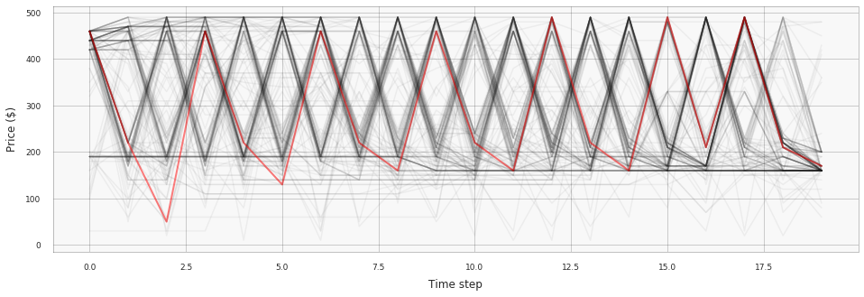
We can see that the result closely resembles the baseline pricing strategy obtained using greedy optimization (but not exactly the same because of randomization). The achieved profit is also very close to the optimum.

The following animation visualizes the same data, but better illustrates how the policy changes over training episodes:

The process starts with a random policy, but the network quickly learns the sawtooth pricing pattern. The following plot shows how returns change during the training process (the line is smoothed using a moving average filter with a window of size 10; the shaded area corresponds to two standard deviations over the window):

Policy visualization, tuning, and debugging

The learning process is very straightforward for our simplistic environment, but policy training can be much more difficult as the complexity of the environment increases. In this section, we discuss some visualization and debugging techniques that can help analyze and troubleshoot the learning process.

One of the most basic things we can do for policy debugging is to evaluate the network for a manually crafted input state and analyze the output Q-values. For example, let us make a state vector that corresponds to time step 1 and an initial price of \$170, then run it through the network:

Capturing Q-values for a given state. Click to expand the code sample.

sample_state = [170, 0, ... ]
Q_s = policy_net(to_tensor(sample_state))
a_opt = Q_s.max(0)[1].detach()        # Optimal price action is price_grid[a_opt]

plt.bar(price_grid, Q_s.detach().numpy(), color='crimson',  width=6, alpha=0.8)

The output distribution of Q-values will be as follows for the network trained without reward discounting (that is, $\gamma=1.00$):

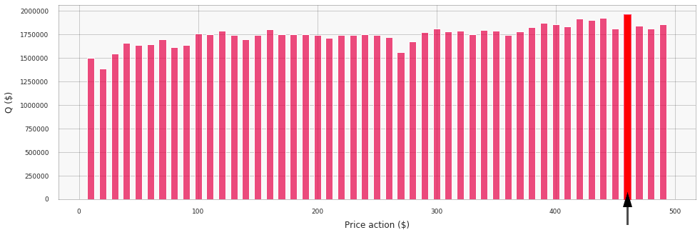
We see that the network correctly suggests increasing the price (in accordance with the Hi-Lo pattern), but the distribution of Q-values if relatively flat and the optimal action is not differentiated well. If we retrain the policy with $\gamma=0.80$, then the distribution of Q-values for the same input state will be substantially different and price surges will be articulated better:

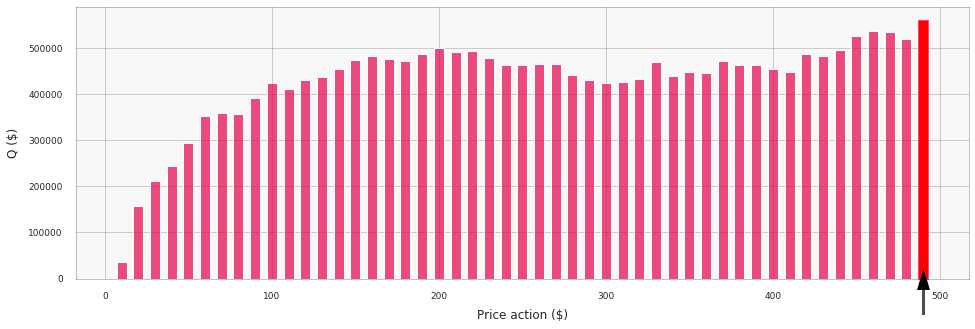
Note that the absolute values of the Q-function do not match the actual return in dollars because of discounting. More specifically, the Q-function now focuses only on the first 10–12 steps after the price action: for example, the discounting factor for 13-th action is $0.8^{13} \approx 0.05$, so its contribution into Q-value is negligible. This often helps to improve the policy or learn it more rapidly because the short-term rewards provide a more stable and predictable guidance for the training process. We can see this clearly by plotting the learning dynamics for two values of $\gamma$ together (note that this plot shows the actual returns, not Q-values, so two lines have the same scale):

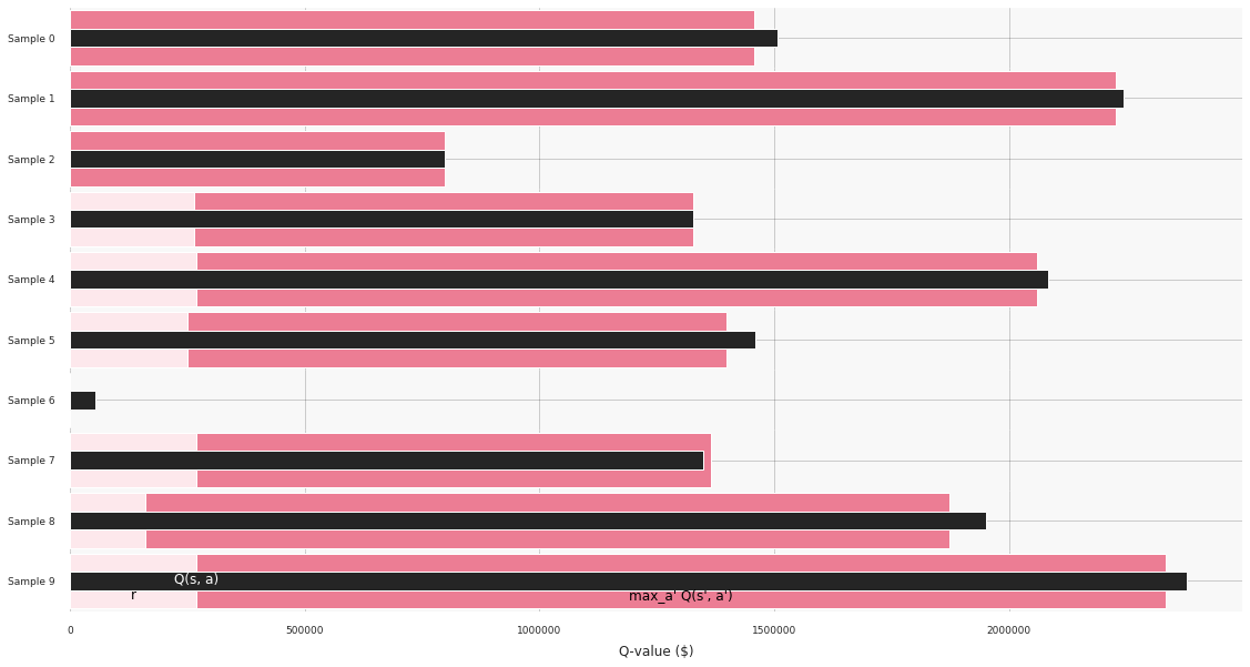
The second technique that can be useful for debugging and troubleshooting is visualization of temporal difference (TD) errors. In the following bar chart, we randomly selected several transitions and visualized individual terms that enter the Bellman equation:

$$
Q(s,a) = r + \gamma\max_{a'} Q(s', a')
$$

The chart shows that TD errors are reasonably small, and the Q-values are meaningful as well:

Finally, it can be very useful to visualize the correlation between Q-values and actual episode returns. The following code snippet shows an instrumented simulation loop that records both values, and the correlation plot is shown right below (white crosses correspond to individual pairs of the Q-value and return).

Correlation between Q-values and actual returns. Click to expand the code sample.

num_episodes = 100
return_trace = []
q_values_rewards_trace = np.zeros((num_episodes, T, 2, ))
for i_episode in range(num_episodes):        # modified copy of the simulation loop
    state = env_intial_state()
    for t in range(T):
        # Select and perform an action
        with torch.no_grad():
          q_values = policy_net(to_tensor(state)).detach().numpy()
        action = policy.select_action(q_values)

        next_state, reward = env_step(t, state, action)

        # Move to the next state
        state = next_state

        q_values_rewards_trace[i_episode][t][0] = q_values[action]   # add the discounted reward to 
        for tau in range(t):                                         # return counters of all previous steps
          q_values_rewards_trace[i_episode][tau][1] += reward * (GAMMA ** (t - tau))

# Visualization
values = np.reshape(q_values_rewards_trace, (num_episodes * T, 2, ))
df = pd.DataFrame(data=values, columns=['Q-value', 'Return'])
sns.jointplot(x="Q-value", y="Return", data=df, kind="kde")

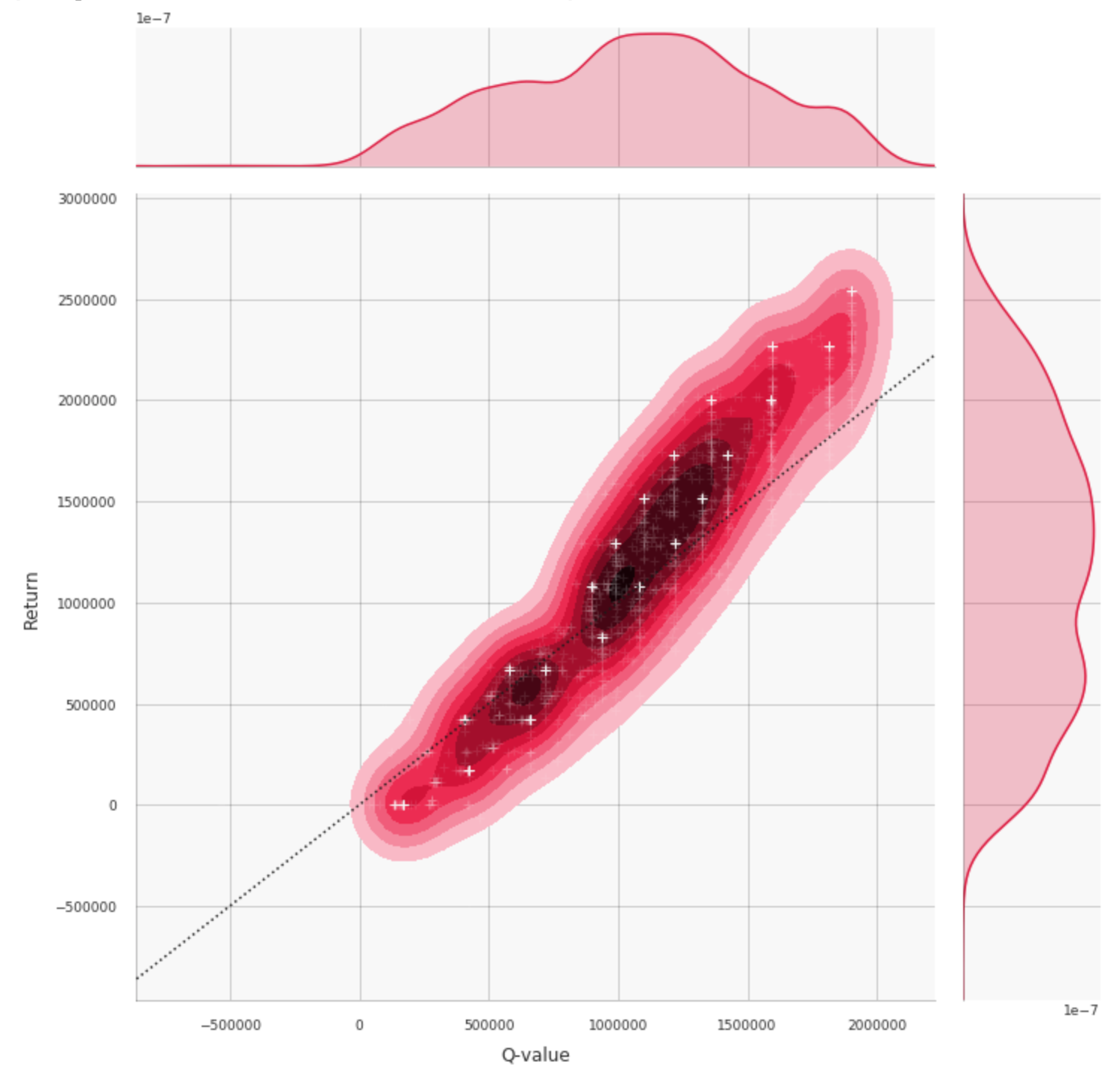
This correlation is almost ideal thanks to the simplicity of the toy price-response function we use. The correlation pattern can be much more sophisticated in more complex environments. A complicated correlation pattern might be an indication that a network fails to learn a good policy, but that is not necessarily the case (i.e., a good policy might have a complicated pattern).

Implementation using RLlib

The DQN implementation we have created in the previous sections can be viewed mainly as an educational exercise. In real industrial settings, it is preferable to use stable frameworks that provide reinforcement learning algorithms and other tools out of the box. Consequently, our next step is to reimplement the same optimizer using RLlib, an open-source library for reinforcement learning developed at the UC Berkeley RISELab ^[6].

We start with the development of a simple wrapper for our environment that casts it to the standard OpenAI Gym interface. We simply need to add a few minor details. First, the environment needs to fully encapsulate the state. Second, dimensionality and type of action and state (observation) spaces have to be explicitly specified:

Pricing environment: Gym wrapper. Click to expand the code sample.

import gym
from gym.spaces import Discrete, Box

class HiLoPricingEnv(gym.Env):
    def __init__(self, config):
        self.reset()
        self.action_space = Discrete(len(price_grid))
        self.observation_space = Box(0, 10000, shape=(2*T, ), dtype=np.float32)

    def reset(self):
      self.state = env_intial_state()
      self.t = 0
      return self.state

    # Returns next state, reward, and end-of-the-episode flag  
    def step(self, action):
      next_state, reward = env_step(self.t, state, action)
      self.t += 1
      self.state = next_state
      return next_state, reward, self.t == T - 1, {}

Once the environment is defined, training the pricing policy using a DQN algorithm can be very straightforward. In our case, it is enough to just specify a few parameters:

Pricing policy optimization using RLlib. Click to expand the code sample.

import ray
import ray.rllib.agents.dqn as dqn

def train_dqn():
  config = dqn.DEFAULT_CONFIG.copy()
  config["log_level"] = "WARN"
  config["train_batch_size"] = 256
  config["buffer_size"] = 10000
  config["hiddens"] = [128, 128, 128]
  trainer = dqn.DQNTrainer(config=config, env=HiLoPricingEnv)
  for i in range(50):
    result = trainer.train()
    print(pretty_print(result))

train_dqn()

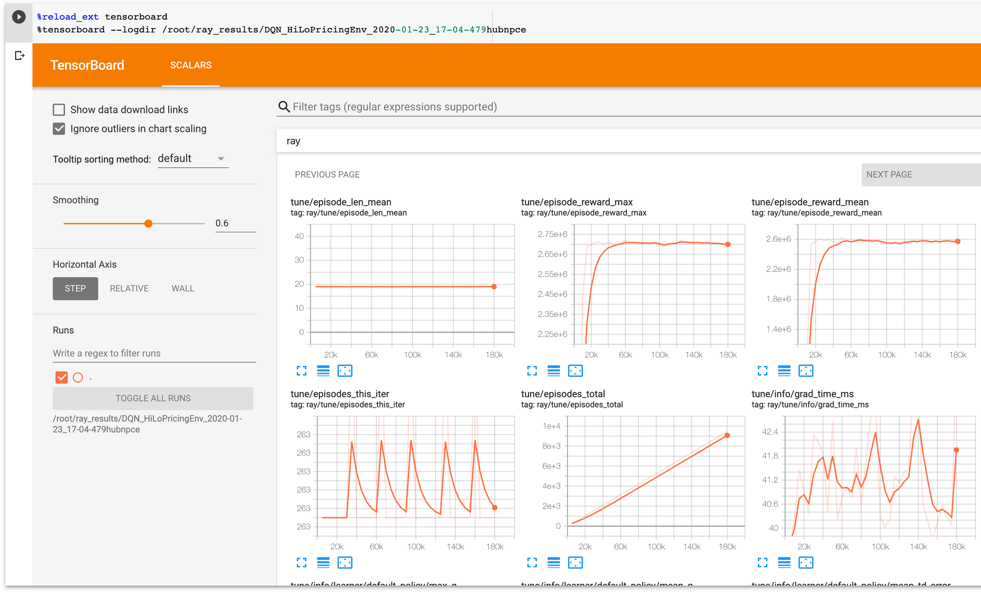
The resulting policy achieves the same performance as our custom DQN implementation. However, RLlib provides many other tools and benefits out of the box such as a real-time integration with TensorBoard:

This concludes our first case study. The solution we developed can work with more complex price-response functions, as well as incorporate multiple products and inventory constraints. We develop some of these capabilities in the next section.

Case study 2: Multi-echelon inventory optimization using DDPG

In the first case study, we discussed how deep reinforcement learning can be applied to the basic revenue management scenario. We also tried out several implementation techniques and frameworks, and we are now equipped to tackle a more complex problem. Our second project will be focused on supply chain optimization, and we will use a much more complex environment with multiple locations, transportation issues, seasonal demand changes, and manufacturing costs.

Defining the environment

We start with defining the environment that includes a factory, central factory warehouse, and $W$ distribution warehouses.^[7][8] An instance of such an environment with three warehouses is shown in the figure below.

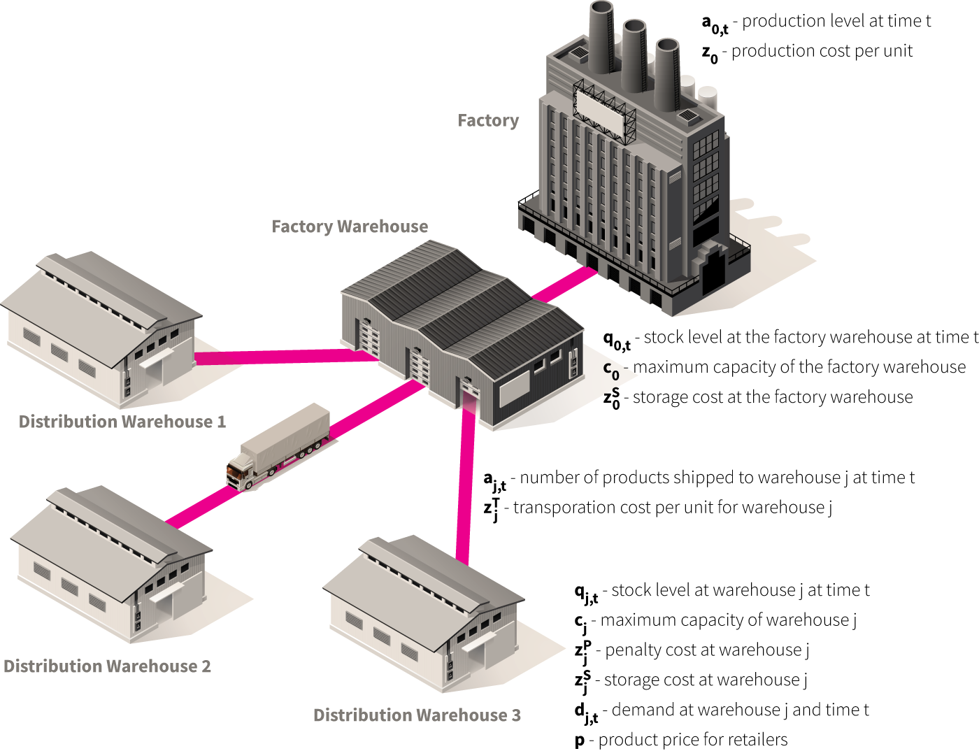
We assume that the factory produces a product with a constant cost of $z_0$ dollars per unit, and the production level at time step $t$ is $a_{0,t}$.

Next, there is a factory warehouse with a maximum capacity of $c_0$ units. The storage cost for one product unit for a one time step at the factory warehouse is $z^S_0$, and the stock level at time $t$ is $s_{0,t}$.

At any time $t$, the number of units shipped from the factory warehouse to the distribution warehouse $j$ is $a_{j,t}$, and the transportation cost is $z^T_{j}$ dollars per unit. Note that the transportation cost varies across the distribution warehouses.

Each distribution warehouse $j$ has maximum capacity $c_j$, storage cost of $z^S_j$, and stock level at time $t$ equal to $q_{j,t}$. Products are sold to retail partners at price $p$ which is the same across all warehouses, and the demand for time step $t$ at warehouse $j$ is $d_{j,t}$ units. We also assume that the manufacturer is contractually obligated to fulfill all orders placed by retail partners, and if the demand for a certain time step exceeds the corresponding stock level, it results in a penalty of $z^P_j$ dollars per each unfulfilled unit. Unfulfilled demand is carried over between time steps (which corresponds to backordering), and we model it as a negative stock level.

Let us now combine the above assumptions together and define the environment in reinforcement learning terms. First, we obtain the following reward function for each time step:

$$
\begin{aligned}
r =\ & p\sum_{j=1}^W d_j - z_0 a_0 -\sum_{j=0}^W z^S_j \max{q_j, 0}\ - \sum_{j=1}^W z^T_j a_j + \sum_{j=1}^W z^P_j\min{q_j, 0}
\end{aligned}
$$

The first term is revenue, the second corresponds to production cost, the third is the total storage cost, and the fourth is the transportation cost. The last term corresponds to the penalty cost and enters the equation with a plus sign because stock levels would be already negative in case of unfulfilled demand.

We choose the state vector to include all current stock levels and demand values for all warehouses for several previous steps:

$$
\begin{aligned}
s_t &= \left( q_{0, t},\ q_{1, t},\ \ldots,\ q_{W, t},\ d_{t-1},\ \ldots, d_{t-\tau} \right) \\
\text{where}\\
d_t &= \left( d_{1,t},\ \ldots,\ d_{W, t}\right)
\end{aligned}
$$

Note that we assume that the agent observes only past demand values, but not the demand for the current (upcoming) time step. This means that the agent can potentially benefit from learning the demand pattern and embedding the demand prediction capability into the policy.

The state update rule will then be as follows:

$$
\begin{aligned}
s_{t+1} = ( &\min\left[q_{0,t} + a_0 - \sum_{j=1}^W a_j,\ c_0\right], &\quad \text{(factory stock update)} \\
& \min\left[q_{1, t} + a_{1, t} - d_{1, t},\ c_1 \right], &\quad \text{(warehouse stock update)} \\
& \ldots, \\
& \min\left[q_{W, t} + a_{W, t} - d_{W, t},\ c_W \right], &\quad \text{(warehouse stock update)} \\
& d_t,\\
& \ldots, \\
& d_{t-\tau} )
\end{aligned}
$$

Finally, the action vector simply consists of production and shipping controls:

$$
a_t = \left( a_{0,t},\ \ldots,\ a_{W,t} \right )
$$

The code snippet below shows the implementation of the state and action classes (see the complete notebook for implementation details).

Supply chain environment: State and action. Click to expand the code sample.

class State(object):
    def __init__(self, warehouse_num, T, demand_history, t = 0):
        self.warehouse_num = warehouse_num
        self.factory_stock = 0
        self.warehouse_stock = np.repeat(0, warehouse_num)
        self.demand_history = demand_history
        self.T = T   # Length of one episode
        self.t = t

    def to_array(self):
        return np.concatenate( ([self.factory_stock], 
                                self.warehouse_stock, 
                                np.hstack(self.demand_history), 
                                [self.t]) )

    def stock_levels(self):
        return np.concatenate( ([self.factory_stock], self.warehouse_stock) )

class Action(object):
    def __init__(self, warehouse_num):
        self.production_level = 0
        self.shippings_to_warehouses = np.zeros(warehouse_num)

The next code snippet shows how the environment is initialized. We assume episodes with 26 time steps (e.g., weeks), three warehouses, and store and transportation costs varying significantly across the warehouses.

Supply chain environment: Initialization. Click to expand the code sample.

class SupplyChainEnvironment(object):
    def __init__(self):
        self.T = 26               # Episode duration
        self.warehouse_num = 3  
        self.d_max = 5            # Maximum demand, units
        self.d_var = 2            # Maximum random demand variation, units 
    
        self.unit_price = 100     # Unit price in dollars
        self.unit_cost = 40       # Unit cost in dollars

        self.storage_capacities = np.fromfunction(lambda j: 10*(j+1), 
                                  (self.warehouse_num + 1,))

        # Storage costs at the factory and each warehouse, dollars per unit
        self.storage_costs = np.fromfunction(lambda j: 2*(j+1), (self.warehouse_num + 1,))
        
        # Transportation costs for each warehouse, dollars per unit   
        self.transporation_costs = np.fromfunction(lambda j: 5*(j+1), (self.warehouse_num,))               
        
        self.penalty_unit_cost = self.unit_price

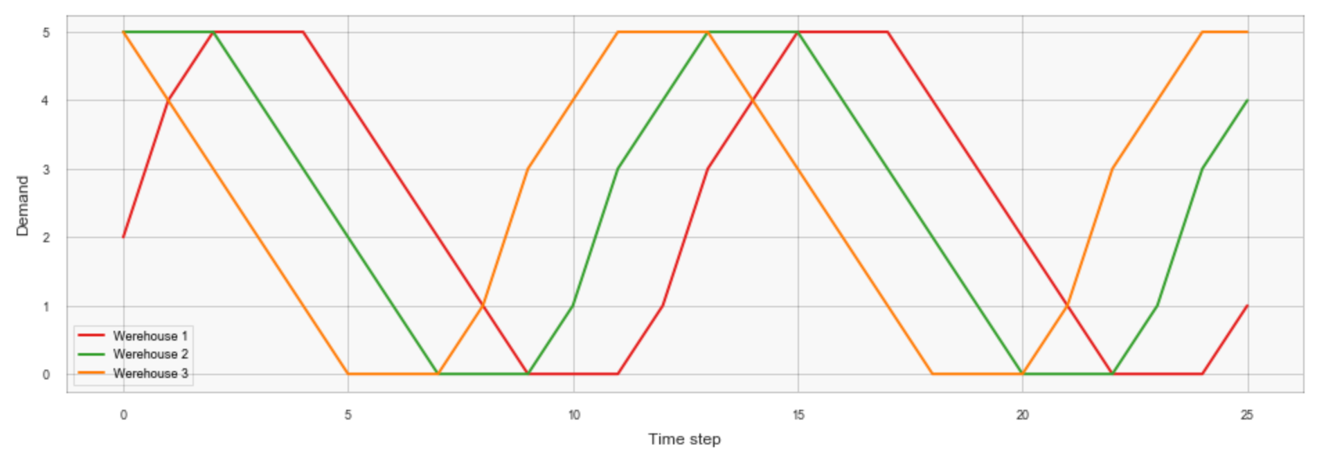
We also define a simple demand function that simulates seasonal demand changes and includes a stochastic component:

$$
d_{j, t} = \frac{d_{max}}{2} \left(1 + \sin\left( \frac{4\pi(t+2j)}{T} \right ) \right ) + \eta_{j,t}
$$

where $\eta$ is a random variable with a uniform distribution. This function is implemented below:

Supply chain environment: Demand function. Click to expand the code sample.

class SupplyChainEnvironment(object):
    ...
    def demand(self, j, t):             # Demand at warehouse j at time t
        return np.round(self.d_max/2 + 
                        self.d_max/2*np.sin(2*np.pi*(t + 2*j)/self.T*2) + 
                        np.random.randint(0, self.d_var))

Finally, we have to implement the state transition logic according to the specifications for reward and state we defined earlier in this section. This part is very straightforward: we just convert formulas for profit and state updates into the code.

Supply chain environment: Transition function. Click to expand the code sample.

class SupplyChainEnvironment(object):
    ...
    def step(self, state, action):
        demands = np.fromfunction(lambda j: self.demand(j+1, self.t), (self.warehouse_num,))
    
        # Calculating the reward (profit)
        total_revenue = self.unit_price * np.sum(demands)
        total_production_cost = self.unit_cost * action.production_level
        total_storage_cost = np.dot( self.storage_costs, 
                np.maximum(state.stock_levels(), np.zeros(self.warehouse_num + 1)) )
        total_penalty_cost = - self.penalty_unit_cost * ( 
                               np.sum( np.minimum(state.warehouse_stock,
                                                  np.zeros(self.warehouse_num)) )  +  
                               min(state.factory_stock, 0) )
        total_transportation_cost = np.dot( self.transporation_costs,               
                                            action.shippings_to_warehouses )
        reward = total_revenue - total_production_cost - total_storage_cost 
                               - total_penalty_cost - total_transportation_cost

        # Calculating the next state
        next_state = State(self.warehouse_num, self.T, self.t)
        next_state.factory_stock = min(state.factory_stock + action.production_level - 
                                       np.sum(action.shippings_to_warehouses), 
                                       self.storage_capacities[0]) 
        for w in range(self.warehouse_num):
            next_state.warehouse_stock[w] = min(state.warehouse_stock[w] + 
                                                action.shippings_to_warehouses[w] - 
                                                demands[w], self.storage_capacities[w+1])    
        next_state.demand_history = list(self.demand_history)

        self.t += 1
        self.demand_history.append(demands)

        return next_state, reward, self.t == self.T - 1

For the sake of simplicity, we assume that fractional amounts of the product can be produced or shipped (alternatively, one can think of it as measuring units in thousands or millions, so that rounding errors are immaterial).

Establishing the baselines

We have defined the environment, and now we need to establish some baselines for the supply chain control policy. One of the traditional solutions is the (s, Q)-policy. This policy can be expressed as the following simple rule: at every time step, compare the stock level with the reorder point $s$, and reorder $Q$ units if the stock level drops below the reorder point or take no action otherwise. This policy typically results in a sawtooth stock level pattern similar to the following:

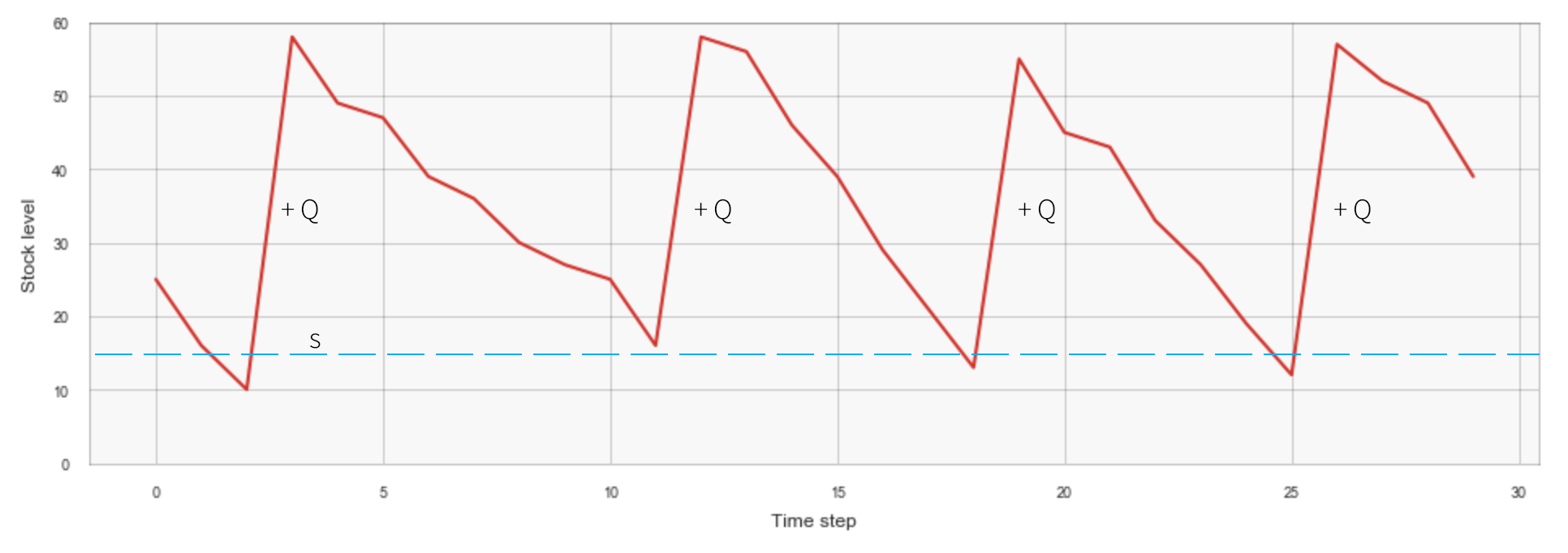
Reordering decisions are made independently for each warehouse, and policy parameters $s$ and $Q$ can be different for different warehouses. We implement the (s,Q)-policy, as well as a simple simulator that allows us to evaluate this policy, in the code snippet below:

(s,Q)-policy and simulator. Click to expand the code sample.

class SQPolicy(object):
    def __init__(self, factory_safety_stock, 
                 factory_reorder_amount, safety_stock, reorder_amount):
        self.factory_safety_stock = factory_safety_stock
        self.factory_reorder_amount = factory_reorder_amount
        self.safety_stock = safety_stock
        self.reorder_amount = reorder_amount

    def select_action(self, state):
        action = Action(state.warehouse_num)
        for w in range(state.warehouse_num):
            if state.warehouse_stock[w] < self.safety_stock[w]:
                action.shippings_to_warehouses[w] = self.reorder_amount[w]
    
        if state.factory_stock - np.sum(action.shippings_to_warehouses) < self.factory_safety_stock: 
            action.production_level = self.factory_reorder_amount
        else: 
            action.production_level = 0
        return action
    
def simulate_episode(env, policy):
    state = env.initial_state()
    transitions = []
    for t in range(env.T):
        action = policy.select_action(state)
        state, reward, _ = env.step(state, action)
        transitions.append([state, action, reward])
    return transitions

# Basic policy evaluation process 
def simulate(env, policy, num_episodes):
    returns_trace = []
    for episode in range(num_episodes):
        env.reset()
        returns_trace.append( sum(np.array(simulate_episode(env, policy)).T[2]) )
    return returns_trace

Setting policy parameters represents a certain challenge because we have 8 parameters, i.e., four (s,Q) pairs, in our environment. In general, the parameters have to be set in a way that balances storage and shortage costs under the uncertainty of the demand (in particular, the reorder point has to be chosen to absorb demand shocks to a certain degree). This problem can be approached analytically given that the demand distribution parameters are known, but instead we take a simpler approach here and do a brute force search through the parameter space using the Adaptive Experimentation Platform developed by Facebook ^[9]. This framework provides a very convenient API and uses Bayesian optimization internally. The code snippet below shows how exactly the parameters of the (s,Q)-policy are optimized:

Optimization of (s, Q)-policy parameters. Click to expand the code sample.

from ax import optimize

def evaluate_sQPolicy(p):
    policy = SQPolicy(
        p['factory_s'], 
        p['factory_Q'],
        [ p['w1_s'], p['w2_s'], p['w3_s'], ],
        [ p['w1_Q'], p['w2_Q'], p['w3_Q'], ]
    )
    return np.mean(simulate(env, policy, num_episodes = 30))

best_parameters, best_values, experiment, model = optimize(
        parameters=[
          { "name": "factory_s",   "type": "range",  "bounds": [0.0, 30.0], },
          { "name": "factory_Q",   "type": "range",  "bounds": [0.0, 30.0], },
          { "name": "w1_s",        "type": "range",  "bounds": [0.0, 20.0], },
          { "name": "w1_Q",        "type": "range",  "bounds": [0.0, 20.0], },  
          { "name": "w2_s",        "type": "range",  "bounds": [0.0, 20.0], },
          { "name": "w2_Q",        "type": "range",  "bounds": [0.0, 20.0], },    
          { "name": "w3_s",        "type": "range",  "bounds": [0.0, 20.0], },
          { "name": "w3_Q",        "type": "range",  "bounds": [0.0, 20.0], },    
        ],
        evaluation_function=evaluate_sQPolicy,
        minimize=False,
        total_trials=200,
    )

We combine this optimization with grid search fine tuning to obtain the following policy parameters and achieve the following profit performance:

Optimized policy parameters:
Factory (s, Q) = (0, 20)
Warehouse 1 (s, Q) = (5, 5)
Warehouse 2 (s, Q) = (5, 5)
Warehouse 3 (s ,Q) = (5, 10)

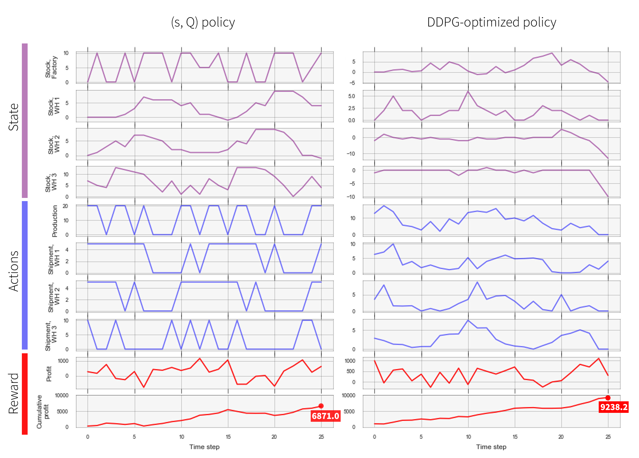
Achieved profit: 6871.0

We can get more insight into the policy behavior by visualizing how the stock levels, shipments, production levels, and profits change over time:

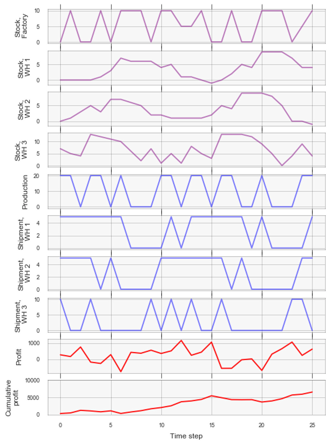
In our testbed environment, the random component of the demand is relatively small, and it makes more sense to ship products on an as-needed basis rather than accumulate large safety stocks in distribution warehouses. This is clearly visible in the above plots: the shipment patterns loosely follow the oscillating demand pattern, while stock levels do not develop a pronounced sawtooth pattern.

Overview of the DDPG algorithm

We now turn to the development of a reinforcement learning solution that can outperform the (s,Q)-policy baseline. Our supply chain environment is substantially more complex than the simplistic pricing environment we used in the first part of the tutorial, but, in principle, we can consider using the same DQN algorithm because we managed to reformulate the problem in reinforcement learning terms. The issue, however, is that DQN generally requires a reasonably small discrete action space because the algorithm explicitly evaluates all actions to find the one that maximizes the target Q-value (see step 2.3.2 of the DQN algorithm described earlier):

$$
y_i = r_i + \gamma\max_{a'} Q^{\pi_\theta}(s', a')
$$

This was not an issue in our first project because the action space was defined as a set of discrete price levels. In the supply chain environment, an action is a vector of production and shipping controls, so the action space grows exponentially with the size of the chain, and we also allow controls to be real numbers, so the action space is continuous. In principle, we can work around this through discretization. For example, we can allow only three levels for each of four controls, which results in $3^4 = 81$ possible actions. This approach, however, is not scalable. Fortunately, continuous control is a well-studied problem and there exists a whole range of algorithms that are designed to deal with continuous action spaces. We choose to use Deep Deterministic Policy Gradient (DDPG), which is one of the state-of-the-art algorithms suitable for continuous control problems ^[10][11]. It is more complex than DQN, so we will review it only briefly, while more theoretical and implementation details can be found in the referenced articles.

Policy gradient. DQN belongs to the family of Q-learning algorithms. The central idea of Q-learning is to optimize actions based on their Q-values, and thus all Q-learning algorithms explicitly learn or approximate the value function. The second major family of reinforcement learning algorithms is policy gradient algorithms. The central idea of the policy gradient is that the policy itself is a function with parameters $\theta$, and thus this function can be optimized directly using gradient descent. We can express this more formally using the following notation for the policy:

$$
\pi_\theta(s) \rightarrow a
$$

We are generally interested in finding the policy that maximizes the average return $R$, so we define the following objective function:

$$
J(\pi_\theta) = E_{s,a,r\ \sim\ \pi_\theta}[R]
$$

The policy gradient solves the following problem:

$$
\max_\theta J(\pi_\theta)
$$

using, for example, gradient ascent to update the policy parameters:

$$
\theta \leftarrow \theta + \alpha \nabla_\theta J(\pi_\theta)
$$

The most straightforward way to implement this idea is to compute the above gradient directly for each observed episode and its return (which is known as the REINFORCE algorithm). This is not particularly efficient because the estimates computed based on individual episodes are generally noisy, and each episode is used only once and then discarded. On the other hand, the policy gradient is well suited for continuous action spaces because individual actions are not explicitly evaluated.

Actor-Critic: Combining policy gradient with Q-learning. The limitation of the basic policy gradient, however, can be overcome through combining it with Q-learning, and this approach is extremely successful. The main idea is that it can be more beneficial to compute the policy gradient based on learned value functions rather than raw observed rewards and returns. This helps to reduce the noise and increase robustness of the algorithm because the learned Q-function is able to generalize and “smooth” the observed experiences. This leads to the third family of algorithms known as Actor-Critic. All these algorithms have a dedicated approximator for the policy (actor) and the second approximator that estimates Q-values collected under this policy (critic).

The DDPG algorithm further combines the Actor-Critic paradigm with the stabilization techniques introduced in DQN: an experience replay buffer and target networks that allow for complex neural approximators. Another important aspect of DDPG is that it assumes a deterministic policy $\pi(s)$, while the traditional policy gradient methods assume stochastic policies that specify probabilistic distributions over actions $\pi(a | s)$. The deterministic policy approach has performance advantages and is generally more sample-efficient because the policy gradient integrates only over state space, but not action space. The pseudocode below shows how all these pieces fit together:

Note that the gradient ascent update for the actor is based on the Q-function approximation, not on the original transitions. DDPG also uses soft updates (incremental blending) for the target networks, as shown in step 2.3.5, while DQN uses hard updates (replacement).

Implementation using RLlib

Our last step is to implement training of the supply chain management policy using RLlib. We first create a simple Gym wrapper for the environment we previously defined:

Supply chain environment: Gym wrapper. Click to expand the code sample.

class SimpleSupplyChain(gym.Env):
    def __init__(self, config):
        self.reset()
        self.action_space = Box(low=0.0, high=20.0)            # Continuous space
        self.observation_space = Box(low=-10000, high=10000)

    def reset(self):
        self.supply_chain = SupplyChainEnvironment()
        self.state = self.supply_chain.initial_state()
        return self.state.to_array()

    def step(self, action):
        action_obj = Action(self.supply_chain.warehouse_num)
        action_obj.production_level = action[0]
        action_obj.shippings_to_warehouses = action[1:]
        self.state, reward, done = self.supply_chain.step(self.state, action_obj)
        return self.state.to_array(), reward, done, {}

Next, we implement the training process using RLlib, which is also very straightforward:

Supply chain optimization using RLlib and DDPG. Click to expand the code sample.

config = ddpg.DEFAULT_CONFIG.copy()
config["actor_hiddens"] = [512, 512] 
config["critic_hiddens"] = [512, 512]
config["gamma"] = 0.95
config["timesteps_per_iteration"] = 1000
config["target_network_update_freq"] = 5
config["buffer_size"] = 10000
    
trainer = ddpg.DDPGTrainer(config=config, env=SimpleSupplyChain)
for i in range(n_iterations):
   result = trainer.train()
   print(pretty_print(result))
  
#> Achieved profit: 9238.2

The policy trained this way substantially outperforms the baseline (s, Q)-policy. The figure below shows example episodes for two policies compared side by side:

In principle, it is possible to combine DDPG with parametric inventory management models like (s,Q)-policy in different ways. For example, one can attempt to optimize reorder points and amount parameters of the (s,Q) policy using DDPG.

Deep reinforcement learning for enterprise operations

We conclude this article with a broader discussion of how deep reinforcement learning can be applied in enterprise operations: what are the main use cases, what are the main considerations for selecting reinforcement learning algorithms, and what are the main implementation options.

Use cases. Most enterprise use cases can be approached from both myopic (single stage) and strategic (multi-stage) perspectives. This can be illustrated by the following examples:

• Traditional price optimization focuses on estimating the price-demand function and determining the profit-maximizing price point. In the strategic context, one would consider a sequence of prices and inventory movements that must be optimized jointly.
• Traditional personalization models are trained to optimize the click-through rate, conversion rate, or other myopic metrics. In the strategic context, a sequence of multiple marketing actions has to be optimized to maximize customer lifetime value or a similar long-term objective.

Reinforcement learning is a natural solution for strategic optimization, and it can be viewed as an extension of traditional predictive analytics that is usually focused on myopic optimization. Reinforcement learning is also a natural solution for dynamic environments where historical data is unavailable or quickly becomes obsolete (e.g., newsfeed personalization).

Action space. Some enterprise use cases can be better modeled using discrete action spaces, and some are modeled using continuous action spaces. This is a major consideration for selecting a reinforcement learning algorithm. The DQN family (Double DQN, Dueling DQN, Rainbow) is a reasonable starting point for discrete action spaces, and the Actor-Critic family (DDPG, TD3, SAC) would be a starting point for continuous spaces.

On-policy vs. off-policy. In many reinforcement learning problems, one has access to an environment or simulator that can be used to sample transitions and evaluate the policy. Typical examples include video game simulators, car driving simulators, and physical simulators for robotics use cases. This can be an option for enterprise use cases as well. For instance, we previously created a supply chain simulator. However, many enterprise use cases do not allow for accurate simulation, and real-life policy testing can also be associated with unacceptable risks. Marketing is a good example: although reinforcement learning is a very compelling option for strategic optimization of marketing actions, it is generally not possible to create an adequate simulator for a customer behavior, and random messaging to the customers for policy training or evaluation is also not feasible. In such cases, one has to learn offline-based historical data and carefully evaluate a new policy before deploying it to production. It is not trivial to correctly learn and evaluate a new policy having only the data collected under some other policy (off-policy learning), and this problem is one the central challenges for enterprise adoption of reinforcement learning.

Single-agent vs. multi-agent. Most innovations and breakthroughs in reinforcement learning in recent years have been achieved in single-agent settings. However, many enterprise use cases, including supply chains, can be more adequately modeled using the multi-agent paradigm (multiple warehouses, stores, factories, etc.). The choice of algorithms and frameworks is somewhat more limited in such a case.

Perception vs combinatorial optimization. The success of deep reinforcement learning largely comes from its ability to tackle problems that require complex perception, such as video game playing or car driving. The applicability of deep reinforcement learning to traditional combinatorial optimization problems has been studied as well, but less thoroughly ^[12]. Many enterprise use cases, including supply chains, require combinatorial optimization, and this is an area of active research for reinforcement learning.

Technical platform. There are a relatively large number of technical frameworks and platforms for reinforcement learning, including OpenAI Baselines, Berkeley RLlib, Facebook ReAgent, Keras-RL, and Intel Coach. Many of these frameworks provide only algorithm implementations, but some of them are designed as platforms that are able to learn directly from system logs and essentially provide reinforcement learning capabilities as a service. This latter approach is very promising in the context of enterprise operations.

References

---

1. Mnih V., et al. "Human-level control through deep reinforcement learning", 2015 ↩︎ ↩︎

2. Hessel M., et al. “Rainbow: Combining Improvements in Deep Reinforcement Learning,” 2017 ↩︎

3. Graesser L., Keng W. L., Foundations of Deep Reinforcement Learning, 2020 ↩︎

4. Sutton R., Barto A., Reinforcement Learning, 2018 ↩︎

5. Reinforcement Learning (DQN) Tutorial ↩︎

6. RLlib: Scalable Reinforcement Learning ↩︎

7. Kemmer L., et al. “Reinforcement learning for supply chain optimization,” 2018 ↩︎

8. Oroojlooyjadid A., et al. “A Deep Q-Network for the Beer Game: Reinforcement Learning for Inventory Optimization,” 2019 ↩︎

9. Adaptive Experimentation Platform ↩︎

10. Silver D., Lever G., Heess N., Degris T., Wierstra D., Riedmiller M. “Deterministic Policy Gradient Algorithms,” 2014 ↩︎

11. Lillicrap T., Hunt J., Pritzel A., Heess N., Erez T., Tassa Y., Silver D., Wierstra D., “Continuous control with deep reinforcement learning,” 2015 ↩︎

12. Bello I., Pham H., Le Q., Norouzi M., Bengio S. “Neural Combinatorial Optimization with Reinforcement Learning,” 2017 ↩︎