A guide to dynamic pricing algorithms

The ability to generate optimal prices is key for retail, because price-setting errors directly lead to lost profits. However, traditional pricing strategies nowadays rarely result in setting optimal prices since they are designed for more traditional environments. In such environments, the price change frequency is inherently limited (for example, brick-and-mortar stores), and off-the-shelf tool capabilities and manual processes constrain the ability to use dynamic pricing models.

Dynamic pricing algorithms, on the other hand, enable adjusting prices frequently and collecting real-time data for repricing scenarios and thus help increase the quality of e-commerce pricing decisions. These capabilities bring significant benefits to the company:

1. Unlock more efficient response to demand changes;
2. Improve the forecasting model quality by reducing errors;
3. Automate price management for catalogs with hundreds of millions of items.

This article is a technical deep dive into dynamic pricing algorithms that power online sales price ranges for different customer segments. In particular, it covers algorithms that use dynamic pricing reinforcement learning and Bayesian inference ideas, and are tested at scale by companies like Walmart and Groupon.

Dynamic pricing algorithms vs traditional

Traditional price optimization requires knowing or estimating dependency between price and demand. Assuming that this dependency is known (at least for a certain time interval), the following equation can be used to find the revenue-optimal price:
$$
p^* = \underset{p}{\text{argmax}}\ \ p \times d(p)
$$

where $p$ is the price and $d(p)$ is a demand function. Retailers can also incorporate item costs, cross-item demand cannibalization, competitor prices, promo activities, inventory constraints, and many other factors into the basic model. The traditional price management process assumes that the demand function is estimated from the historical sales data. To estimate the function, a regression analysis for observed pairs of prices and corresponding demands $(p_i, d_i)$ is performed. Since the price-demand relationship changes over time, a typical traditional process regularly re-estimates the demand function. This leads to a simplistic dynamic pricing algorithm:

1. Collect historical data at different price points offered in the past as well as the observed demands for these points.
2. Estimate the demand function.
3. Solve the optimization problem, using the historical data as a reference, to find the optimal price that maximizes a metric like revenue or profit margin, and meets the constraints imposed by the pricing policy or inventory.
4. Apply this optimal price for a certain time period, observe the actual demand, and repeat the steps again.

The fundamental limitation of this approach is that it passively learns the demand function without actively exploring the dependency between the price and demand. This might work depending on environment dynamics:

• If the product life cycle is relatively long and the demand function changes relatively slowly, the passive learning approach combined with organic price changes can be efficient, as the price it sets will be close to the true optimal price most of the time.
• If the product life cycle is relatively short or the demand function changes rapidly, the difference between the price produced by the algorithm and the true optimal price can become significant, and so will the lost revenue. In practice, this difference is substantial for many online retailers, and critical for retailers that extensively rely on short-time offers or flash sales (Groupon, Rue La La, etc.)

The second case represents a classical exploration-exploitation problem of dynamic environments. It is crucial to shorten the cycles of testing different price levels and collecting the corresponding demand points to accurately estimate the demand curve, while maximizing the time used to sell at the optimal price calculated based on the estimate.
That is why we decided to design a solution that optimizes this trade-off while complying to real-life constraints. More specifically, the goals include:

1. Optimize the exploration-exploitation trade-off given that the seller does not know the demand function in advance (for example, a product is new and there is no historical data on it). This trade-off can be quantified as the difference between the actual revenue and the hypothetically possible revenue given that the demand function is known.
2. Provide the ability to limit the number of price changes during the product life cycle. Although the frequency of price changes in digital channels is virtually unlimited, many sellers impose certain limitations to avoid inconsistent customer experience and other issues.
3. Provide the ability to specify valid price levels and price combinations. Most retailers restrict themselves to a certain set of price points (e.g., $25.90, $29.90, ..., $55.90), and the optimization process has to support this constraint.
4. Enable the optimization of prices under inventory constraints, or given dependencies between particular products.

The following sections discuss several techniques for achieving such goals, starting with the most straightforward ones and gradually moving to more sophisticated algorithms that account for a more complex process for pricing decisions.

Scenario 1: Limited price changes and iterative hypotheses

Let’s assume that demand remains constant during the product life cycle, but the seller’s pricing strategy limits the number of price changes. This scenario is often a valid approximation for flash sales or time-limited deals. For instance, Groupon tested a variant of the dynamic pricing described below and achieved very positive results. ^[1]

Assuming that the total duration of the product life cycle $T$ is known to the seller in advance, the goal is to sequentially optimize prices for $m$ time intervals, and also optimize the durations $\tau_i$ of these intervals:

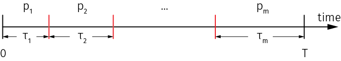
In an extreme case, only one price change is allowed. For example, a seller starts with an initial price guess, collects the demand data during the first period of time (exploration), computes the optimized price, and sells at this new price during the second time period that ends with the end of the product life cycle (exploitation).

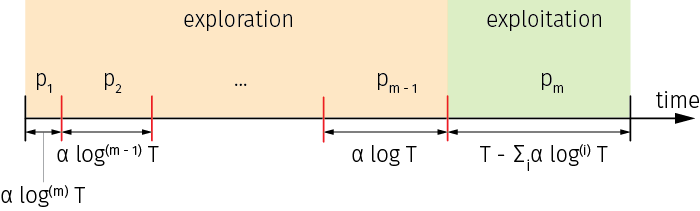
For such circumstances, the optimal price interval durations have to increase exponentially, so that a seller starts with short intervals to explore and learn, and gradually increases the intervals until the final price is set for the last and the longest interval, which is focused purely on exploitation:

$$\tau_i = \alpha \log^{(m-i)}T$$

where $\log^{(n)}x$ stands for $n$ iterations of the logarithm, $\log(\log(...\log x))$, and $\alpha$ is a coefficient that depends on the demand distribution. For practical purposes, $\alpha$ can be chosen empirically because the parameters of the demand may not be known. This layout is illustrated in the figure below:

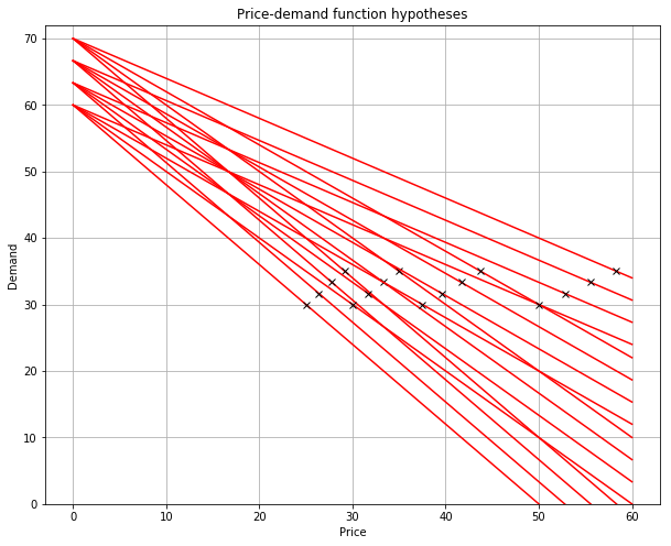
Next, we need to specify how the prices are generated for each time interval. One simple but flexible approach is to generate a set of parametric demand functions (hypotheses) in advance, pick the hypothesis that most closely corresponds to the observed demand at the end of each time interval, and optimize the price for the next interval based on this hypothesis.
In practice, we can generate a set of hypotheses based on the historical demand functions for same or similar products or categories. For this, we need to generate a reasonably dense “grid” of demand curves that covers the range where the true demand function is likely to be located.

Let’s summarize how a complete dynamic pricing algorithm looks:

Implementation of the iterative hypothesis testing

Let's implement the above algorithm and run a simulation. We use a linear demand model to generate the hypotheses (and it is a reasonable choice for many practical applications as well), but any other parametric demand model, such as the constant-elasticity model, can also be used.

For a linear model, the revenue-optimal price can be calculated by taking a derivative of the revenue with respect to price, and equating it to zero: $$
\begin{aligned}
d(p) &= b + a\cdot p \\
p_{\text{opt}} &:\ \frac{\delta}{\delta p}\ p\cdot d(p) = 0 \\
p_{\text{opt}} &= -\frac{b}{2a}
\end{aligned} $$

This logic can be implemented as follows:

def linear(a, b, x):
    return b + a*x

# a linear demand function is generated for every 
# pair of coefficients in vectors a_vec and b_vec 
def demand_hypotheses(a_vec, b_vec):
    for a, b in itertools.product(a_vec, b_vec):
        yield {
            'd': functools.partial(linear, a, b),
            'p_opt': -b/(2*a)
        }

We use this code to generate a sample set of demand functions and the corresponding optimal prices:

For the runtime portion of the algorithm, we generate the price interval schedule in advance, and use it to determine whether we need to generate a new price at every time step (as we mentioned earlier, the schedule depends on the properties of the demand distribution, which are unknown to the seller, so the fixed schedule is a heuristic approximation):

Click to expand the code sample (36 lines)

T = 24 * 1                              # time step is one hour, flash offering for 1 day 
m = 4                                   # not more than 4 price updates

def logx(x, n):                         # iterative logarithm function
    for i in range(0, n): x = math.log(x) if x > 0 else 0
    return x

def intervals(m, T, scale):             # generate a price schedule vector
    mask = []
    for i in range(1, m):
        mask.extend( np.full(scale * math.ceil(logx(T, m - i)), i - 1) )
    return np.append(mask, np.full(T - len(mask), m - 1))

tau = 0                                 # start time of the current interval
p = h_vec[0]['p_opt']                   # initial price

t_mask = intervals(m, T, 2)
h_vec = demand_hypotheses(...)

hist_d = []
for t in range(0, T - 1):               # simulation loop
    realized_d = sample_actual_demand(p)
    hist_d.append(realized_d)

    if( t_mask[t] != t_mask[t + 1] ):   # end of the interval
        interval_mean_d = np.mean( hist_d[tau : t + 1] )
        
        min_dist = float("inf")
        for h in h_vec:                 # search for the best hypothesis
            dist = abs(interval_mean_d - h['d'](p))
            if(dist < min_dist):
                min_error = error
                h_opt = h

        p = h_opt['p_opt']              # set price for the next interval
        tau = t + 1                     # switch to the next interval

The execution of this algorithm is illustrated in the animation below. The top chart shows the true demand function as the dotted line, the realized demands at each time step as red crosses (sampled from the true demand function with additive noise), and the black lines as the selected hypotheses. The bottom plot shows the price and demand for every time step, with the price intervals highlighted with different bar colors.

Scenario 2: Continuous experimentation under pricing rules

In the previous section, we described a simple yet efficient dynamic pricing model for situations, where we can assume the demand function to be stationary. For more dynamic environments, we need to use more generic tools that can continuously explore the environment, while also balancing the exploration-exploitation trade-off. Fortunately, reinforcement learning theory offers a wide range of methods designed specifically for this issue.

In this section, we will discuss a very flexible framework for dynamic pricing that uses reinforcement learning ideas and can be customized to support an extensive range of use cases and constraints.^[2] Walmart tested a variant of this framework with positive results.^[3]

Let's start with an observation that the approach used in Scenario 1 can be improved in the following two areas:

1. We can expect to build a more flexible and efficient framework by utilizing Bayesian methods for demand estimation. Using a Bayesian approach will enable us to accurately update the demand distribution model with every observed sample, as well as quantify the uncertainty in the model parameter estimates.
2. We should replace the fixed price change schedule with continuous exploration. Again, a Bayesian approach can help to better control the exploration process, as the time allocated for exploration and the breadth of exploration can be derived from the uncertainty of the demand estimates.

These two ideas are combined together in Thompson sampling, a generic method that belongs to a large and well-researched family of algorithms for the multi-armed bandit problem (a particular formulation of the exploration-exploitation problem). First, let's review a generic description of the Thompson sampling algorithm for demand estimation, and then refine it with more details:

The main idea of Thompson sampling is to control the amount of exploration by sampling the model parameters for a probabilistic distribution that is refined over time. If the variance of the distribution is high, we will tend to explore a wider range of possible demand functions. If the variance is low, we will mostly use functions that are close to what we think is the most likely demand curve (that is, the curve defined by the mean of the distribution), and explore more distant shapes only occasionally. Note that the demand distribution incorporates both the dependency between the price and demand (which can be composed of deterministic and random components).

To make the above algorithm concrete, we need to specify a probabilistic model for the demand using:

• Linear, constant-elasticity or some other continuous model that treats the slope coefficient or elasticity coefficient as a random parameter θ.
• Model with a discrete set of price levels.
  The latter approach is preferable in many environments because many companies, especially retailers, have a pricing policy that prescribes a certain set of price levels (such as $5.90, $6.90, etc.). The demand model in this case represents a table with $k$ price levels, and each price level is associated with its own demand probability density function (PDF) specified by some parameters, so that the overall demand curve can be visualized by plotting the price levels and their mean demands:

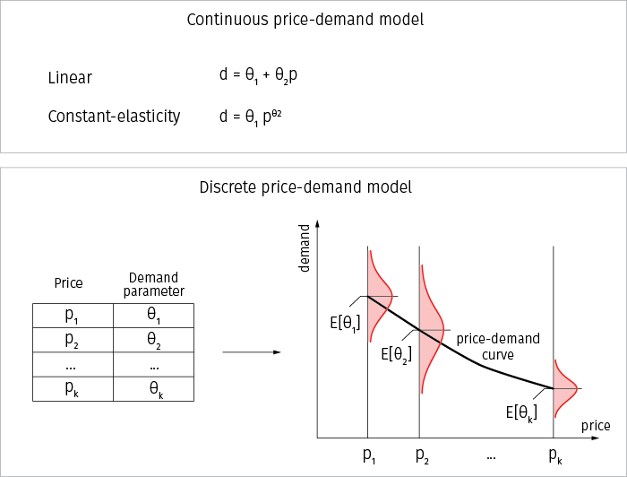
Thus, the curve can have an arbitrary shape and can approximate a wide range of price-demand dependencies, including linear and constant-elasticity models.

Next, we need to specify the demand distributions for individual price levels. For illustrative purposes, we assume that there is no correlation between prices. In this case, parameter $\theta$ can simply be the mean demand at the corresponding price level. In other words, the demand distribution model conditioned on $\theta$ becomes trivial because the shape of the demand curve is already captured point by point, and we can sample the mean demand at each point to optimize the price. Let’s assume that the observed demand samples have a Poisson distribution (a natural choice because each sample represents the number of purchases per unit of time):
$$
d_1, \ldots, d_n \sim \text{poisson}(\theta)
$$

The prior $\theta$ distribution can be chosen to be gamma because it is conjugate to the Poisson distribution:
$$
p(\theta)=\text{gamma}(\alpha, \beta) = \frac{\beta^\alpha}{\Gamma(\alpha)} \theta^{\alpha-1} e^{-\beta\theta}
$$

The likelihood given the observed samples for a certain price is:
$$
p(d\ |\ \theta) = \prod_{i=1}^n \frac{e^{-\theta} \theta^{d_i}}{d_i!} = \frac{e^{-n\theta} \theta^{\sum_i d_i}}{\prod_i d_i!}
$$

Finally, the update rule for the posterior distribution of the parameter $\theta$ is obtained as a product of the prior and likelihood:
$$
p(\theta) \leftarrow p(\theta)\cdot p(d\ |\ \theta) =\text{gamma}(\alpha + \sum d_i,\ \beta+n)
$$

We update the prior distribution at a certain price point by adding the number of times this price was offered to hyperparameter $\beta$, and the total demand observed during these times to the hyperparameter $\alpha$.

Given the above assumptions, we can rewrite the Thompson sampling algorithm as follows:

This version of the algorithm is detailed enough to handle more dynamic pricing, and can be implemented straightforwardly.

Implementation of Thompson sampling for dynamic pricing

Take a look at the algorithm and the parts needed to run a simulation example of a dynamic pricing implementation with Thompson sampling in the code snippet below.

Click to expand the code sample (40 lines)

# parameters
prices = [1.99, 2.49, 2.99, 3.49, 3.99, 4.49]
alpha_0 = 30.00     # parameter of the prior distribution
beta_0 = 1.00       # parameter of the prior distribution

# parameters of the true (unknown) demand model
true_slop = 50
true_intercept = -7

# prior distribution for each price
p_theta = []
for p in prices:
    p_theta.append({'price': p, 'alpha': alpha_0, 'beta': beta_0})

def sample_actual_demand(price): 
    demand = true_slop + true_intercept * price
    return np.random.poisson(demand, 1)[0]

# sample mean demands for each price level
def sample_demands_from_model(p_theta):
    return list(map(lambda v: 
           np.random.gamma(v['alpha'], 1/v['beta']), p_theta))

# return price that maximizes the revenue
def optimal_price(prices, demands):
    price_index = np.argmax(np.multiply(prices, demands))
    return price_index, prices[price_index]

# simulation loop        
for t in range(0, T):
    demands = sample_demands_from_model(p_theta)   
    price_index_t, price_t = optimal_price(prices, demands)
    
    # offer the selected price and observe demand
    demand_t = sample_actual_demand(price_t)
        
    # update model parameters
    v = p_theta[price_index_t]
    v['alpha'] = v['alpha'] + demand_t
    v['beta'] = v['beta'] + 1

By running this implementation and recording how the parameters of the distributions are changing over time, we can observe how the algorithm explores and learns the demand function:

In the beginning, the demand parameters are the same for all price levels. The algorithm actively explores different prices (the red line in the bottom chart), becomes certain that the price of $3.99 provides the best revenue (the yellow curve in the middle chart), and starts to choose it most of the time, exploring other options only occasionally.

We conclude this section with a note that Thompson sampling is not the only choice for dynamic price optimization; there are a wide range of alternative algorithms that can be used in practice, and generic off-the-shelf implementations of such algorithms are readily available.^[4] Many of these algorithms are designed for advanced formulations of multi-armed bandit problems, such as contextual bandit problems, and can improve their performance by using additional pieces of information, such as customer profile data. The basic Thompson sampler can also be extended in many ways (see, for example, ^[5] for a detailed treatment). In particular, we can dramatically increase the flexibility of a demand forecasting model using Markov Chain Monte Carlo (MCMC) methods, as we discuss later in this article.

Scenario 3: Multiple products or time intervals

Let’s consider how we can extend the Scenario 2 framework to support various constraints and features. For example, adding inventory constraints to the routine that finds optimal prices to exclude the options in which demand exceeds the available inventory. The framework can also be extended to estimate demands and optimize prices for multiple products, and optimization typically remains straightforward until dependencies between products or time intervals appear (the optimization problem can be solved separately for each product). Such dependencies can make the optimization problem much more challenging. In this section, we discuss the scenarios with dependencies between products or time intervals, and the optimization methods that can help to handle such use cases.

Consider a scenario where a seller offers multiple products in a category or group, so that the products are fully or partly substitutable. In the general case, the demand function for each product depends on all individual prices of other products. This brings a layer of complexity to accurate estimation and optimization, especially in the dynamic pricing settings. One possible simplification is to use a demand function that depends not on the individual prices of other products, but on the average price within a group of substitutable products.^[6] This can be an accurate approximation in many cases, because the ratio between a product’s own price and the average price in the group reflects the competitiveness of the product and quantifies demand cannibalization. In this case, we can assume a demand model that estimates multiple values for each possible average price instead of separate demand values for each product-price pair (the set of possible average prices is finite because the set of valid price levels is discrete). This assumption leads to the following optimization problem:
$$
\begin{aligned}
\max \ \ & \sum_k \sum_i p_k \cdot d_{ik} \cdot x_{ik} \\
\text{subject to} \ \ & \sum_k x_{ik} = 1, \quad \text{for all } i \\
&\sum_k \sum_i p_k \cdot x_{ik} = c \\
&x_{ik} \in \{0,1\}
\end{aligned}
$$

where $d_{ik}$ is the demand for product $i$, given that it is assigned price $k$, and $x_{ik}$ is a binary dummy variable that is equal to one if price $k$ is assigned to product $i$, and zero otherwise. The first constraint ensures that each product has only one price, and the second constraint ensures that all prices sum up to some value $c$: that is, the average price is fixed. In solving this problem for each possible value of $c$ and picking the best result, we obtain the set of variables $x$ that defines the revenue-optimal assignment of prices to products.

The problem defined above is an integer programming problem, because the decision variables $x$ are either ones or zeros. It can be computationally intractable to solve this problem, even for medium size categories, especially if prices need to be updated frequently. We can work around this problem by replacing the original integer programming problem with a linear programming problem where variables $x$ are assumed to be continuous:
$$
\begin{aligned}
\max \ \ & \sum_k \sum_i p_k \cdot d_{ik} \cdot x_{ik} \\
\text{subject to} \ \ & \sum_k x_{ik} = 1, \quad \text{for all } i \\
&\sum_k \sum_i p_k \cdot x_{ik} = c \\
&0 \le x_{ik} \le 1
\end{aligned}
$$

This technique is known as linear relaxation. The resulting linear program can be solved efficiently, even if the number of products and possible average prices is high. It can be shown that the solution of the linear program gives a good linear bound for the optimal solution of the integer program.^[6:1] This boundary can be used to reduce the set of price sums $c$ for which the integer problem needs to be solved. In practice, the number of integer programs that need to be solved can be reduced significantly (e.g., from hundreds to less than ten).

Another approach is to set prices directly based on the solution of the linear program. In this case, each product can have more than one non-zero variable $x$, and the operational model needs to be adjusted to account for this. For example, a time interval, for which one price is offered, can be divided into multiple sub-intervals in proportion, specified by variables $x$. For instance, if there are two non-zero elements equal to 0.2 and 0.8, then the corresponding prices can be offered for 20% and 80% of the time, respectively.

The approach above using integer programming or linear relaxation can be applied to a range of scenarios, including the following:

• Price optimization for multiple products that have inventory dependencies. For example, a manufacturer can assemble different products from parts drawn from one or several shared pools of resources. In this case, the optimization problem will have a constraint that the total number of parts needed to assemble all products must not exceed the corresponding level of in-stock inventory.
• Price optimization for multiple time intervals. Let’s take into account seasonality of products the retailers purchase at the beginning of the season and have to sell out by the end of the season. In this case, we might be interested not only in the demand forecasting model and optimizing the price for the next time interval. We estimating the demand functions for all time intervals until the end of the season and optimizing prices under the constraint that the sum of the demands for all intervals needs to converge to the available inventory (i.e., the product needs to be sold out or the unsold units will be lost). The optimization problem for one product can then be defined as follows:
  $$
  \begin{aligned}
  \max \ \ & \sum_t \sum_k p_k \cdot d_{tk} \cdot x_{tk} \\
  \text{subject to} \ \ & \sum_k x_{tk} = 1, \quad \text{for all } t \\
  &\sum_t \sum_k d_{tk} \cdot x_{tk} = c \\
  &x_{tk} \in \{0,1\}
  \end{aligned}
  $$
  where $t$ iterates over time intervals within the season.

Implementation of linear relaxation for price optimization

For illustrative purposes, we will implement a solver for the linear relaxation problem with multiple products, as described in the previous section. The solver uses a standard routine for linear programming from the SciPy library that requires the input problem to be defined in the following vector form:
$$
\begin{aligned}
\max \ \ & \mathbf{r} \cdot \mathbf{x} \\
\text{subject to} \ \ & \mathbf{A}\cdot \mathbf{x} = \mathbf{b}
\end{aligned}
$$

We use the following design of the inputs to impose constraints on the sum of the prices and price weights for each product:

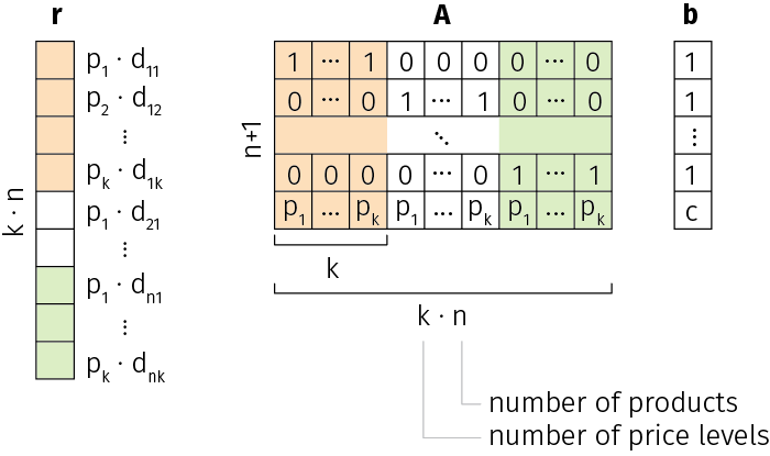
In others words, the cost vector $r$ consists of revenues for all possible price assignments, and each row of matrix $A$ ensures that the price weights sum to 1 for any given product, except the last row that ensures that all prices sum to the required level $c$.

The following code snippet shows the actual implementation and an example test run:

Click to expand the code sample (38 lines)

# prices - k-dimensional vector of allowed price levels 
# demands - n x k matrix of demand predictions
# c - required sum of prices 
# where k is the number of price levels, n is number of products
def optimal_prices_category(prices, demands, c):
    
    n, k = np.shape(demands)  

    # prepare inputs   
    r = np.multiply(np.tile(prices, n), np.array(demands).reshape(1, k*n))
    A = np.array([[
        1 if j >= k*(i) and j < k*(i+1) else 0
        for j in range(k*n)
    ] for i in range(n)])
    A = np.append(A, np.tile(prices, n), axis=0)
    b = [np.append(np.ones(n), c)]

    # solve the linear program
    res = linprog(-r.flatten(), 
              A_eq = A, 
              b_eq = b,  
              bounds=(0, 1))

    np.array(res.x).reshape(n, k)

# test run
optimal_prices_category(
  np.array([[1.00, 1.50, 2.00, 2.50]]),   # allowed price levels
  np.array([
    [ 28, 23, 20, 13],                    # demands for product 1
    [ 30, 22, 16, 12],                    # demands for product 2
    [ 32, 26, 19, 15]                     # demands for product 3
  ]), 5.50)                               # sum of prices for all three products

# output
[[0 0   1 0  ]                            # price vector for product 1 ($2.00)
 [0 1   0 0  ]                            # price vector for product 2 ($1.50)
 [0 0.5 0 0.5]]                           # price vector for product 3 ($1.50 and 2.50)

The algorithm produces a vector of the price weights for each product that can be used to reduce the number of integer programs that need to be solved, or set the prices directly, as described in the previous section.

This solver can be straightforwardly adapted to other cases, such as shared pools of resources or multiple time intervals. Such solvers can then be plugged into any dynamic pricing algorithm described in this article, including the iterative offline learning and Thompson sampling algorithms.

Scenario 4: Complex demand models

Although the demand models used in practice are often simple (linear or constant-elasticity), the development of probabilistic models for Thompson sampling and other similar algorithms can be complicated. Even in our simple implementation of the Thompson sampling algorithm that uses a standard Poisson-Gamma model, we had to do some math and manually implement updated rules for the distribution parameters. This process can be even more complicated if we need to use multivariate distributions for dependent products, or need to customize the model based on business requirements and constraints. We can work around this issue by using probabilistic programming frameworks that allow us to specify models in a declarative manner and abstract the inference procedure. Under the hood, these frameworks use generic MCMC methods to infer the model parameters.

The probabilistic programming approach can be illustrated with a couple of examples that utilize the PyMC3 framework. To start, let's reimplement the Poisson-Gamma model used in Scenario 2 to draw the demand samples:

import pymc3 as pm

d0 = [20, 28, 24, 20, 23]                # observed demand samples

with pm.Model() as m:
    d = pm.Gamma('theta', 1, 1)          # prior distribution
    pm.Poisson('d0', d, observed = d0)   # likelihood
    samples = pm.sample(10000)           # draw samples from the posterior
    
seaborn.distplot(samples.get_values('theta'), fit=stats.gamma)

In the code snippet above, we just declare that the mean demand (theta) has a prior gamma distribution and that the observed demand samples have a Poisson distribution, and point the model to an array with all demand samples observed since selling began. After that, we just draw ten thousand samples from the model, and plot the histogram that follows the posterior distribution of the mean demand:

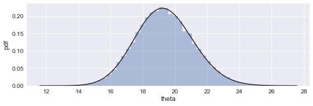
This implementation can be plugged directly into the Thompson sampler, since we associate each price level with an instance of the above model, and draw one sample from each of these models at every time step to solve the price optimization problem. This is a striking simplification compared to the manual updates of the posterior distribution parameters we implemented in the Scenario 2.

We can use the flexibility of this approach to sample the parameters needed for the Thompson sampler from more complex demand models, both discrete and continuous. As a second example, consider a constant-elasticity model defined as follows:
$$
d(p) = b\cdot p^a
$$

We first rewrite this model in the additive (logarithmic) form for the sake of computational stability and ease of modification:^[7]
$$
\log d(p) = \log b + a \log p
$$

The implementation of this model with PyMC3 is straightforward (although we omit some details, such as data centering, for the sake of simplicity):

p0 = [15, 14, 13, 12, 11]    # offered prices
d0 = [20, 28, 35, 50, 65]    # observed demands (for each offered price)

with pm.Model() as m:
    # priors
    log_b = pm.Normal('log_b', sd = 5)
    a = pm.Normal('a', sd = 5)

    log_d = log_b + a * np.log(p0)                    # demand model
    pm.Poisson('d0', np.exp(log_d), observed = d0)    # likelihood
    s = pm.sample()                                   # inference

We can now sample the parameters of the constant-elasticity model, and visualize multiple realizations of the demand function as follows:

p = np.linspace(10, 16)   # price range
d_means = np.exp(s.log_b + s.a * np.log(p).reshape(-1, 1))

plt.plot(p, d_means, c = 'k', alpha = 0.01)
plt.plot(p0, d0, 'o', c = 'r')
plt.show()

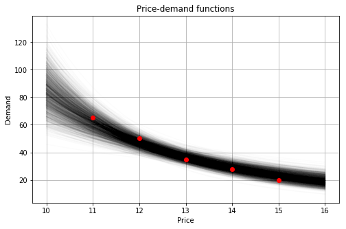
This approach can help to build and test even more complex demand models. It can be particularly useful for multiple related products with correlated demand functions. In this case, the correlated parameters of different demands (e.g., elasticity coefficients) can be drawn from a single multivariate distribution, and probabilistic programming frameworks can significantly help to specify and infer such hierarchical models.

Conclusion: maximize revenue and stay on top of market trends

This article describes several algorithms and techniques that address different aspects of dynamic pricing — experimentation and active learning, dynamic pricing optimization with and without pricing policy constraints, and demand modeling. These methods together constitute a comprehensive toolkit that can be used to build a dynamic pricing engine and customize it based on business requirements and needs.

In practice, dynamic pricing techniques may have a major impact on sales volume and revenue. It is not unusual to see revenue uplift in the range of 10 to 20 percent, and sales volume uplift as high as 80 to 200 percent depending on the product category and business model.^[1:1][2:1] This is the reason that many retailers, including market leaders such as Amazon and Walmart, extensively research and utilize dynamic pricing models, which, in turn, has heavily influenced the retail market as a whole, driving the frequency of price changes up over the last decade.^[8] This makes retail price management increasingly more challenging, and has made algorithmic price management methods, including dynamic pricing and predictive analytics, become an increasingly important source of competitive advantage.

Additionally, the price optimization that takes customer behavior into account can increase customer loyalty with personalized pricing based on machine learning and rich data. Moreover, let’s consider a solution that is based on machine learning algorithms. Initial expectations within the unified basic pattern can take into account competitor prices, SKU-centric or portfolio-based pricing, and then analyze purchasing power of different customers or any other factors into core estimation. Sounds exciting, doesn’t it?

Get in touch to see how economic theory and dynamic pricing models, powered by artificial intelligence and machine learning, can work for your business, increasing customer satisfaction and reducing inventory costs at the same time.

References

---

1. W. Cheung, D. Simchi-Levi, and H. Wang, Dynamic Pricing and Demand Learning with Limited Price Experimentation, February 2017 ↩︎ ↩︎

2. K. Ferreira, D. Simchi-Levi, and H. Wang, Online Network Revenue Management Using Thompson Sampling, November 2017 ↩︎ ↩︎

3. R. Ganti, M. Sustik, T. Quoc, B. Seaman, Thompson Sampling for Dynamic Pricing, February 2018 ↩︎

4. https://github.com/david-cortes/contextualbandits ↩︎

5. D. Russo, B. Roy, A. Kazerouni, I. Osband, Z. Wen, A Tutorial on Thompson Sampling, November 2017 ↩︎

6. K. J. Ferreira, B. Lee, and D. Simchi-Levi, Analytics for an Online Retailer: Demand Forecasting and Price Optimization, November 2015 ↩︎ ↩︎

7. C. Scherrer, Bayesian Optimal Pricing, May 2018 ↩︎

8. A. Cavallo, More Amazon Effects: Online Competition and Pricing Behaviors, September 2018 ↩︎