
A guide to interpretable forecasting models
Forecasting is ubiquitous in modern enterprise operations — a wide range of tasks, from inventory management and price optimization to workforce allocation and equipment maintenance, cannot be efficiently performed without data-driven forecasting. In many of these applications, one needs to not only predict certain metrics or events but also understand the factors that influence the observed time series, estimate the parameters of the underlying processes, and gauge uncertainties and risks. In some applications, such analysis plays a central role and can be more important than forecasting itself. This article is a hands-on tutorial on the methods and techniques that help to analyze the internal structure of typical enterprise time series and gain additional insights from commonly used forecasting models.
Time Series Forecasting and Decomposition in Enterprise Applications
We focus on a simple setup that mimics several important properties of real-life enterprise time series such as sales data. Let us assume an observed signal that includes hidden trend, seasonality, and noise components as well as observed covariates:
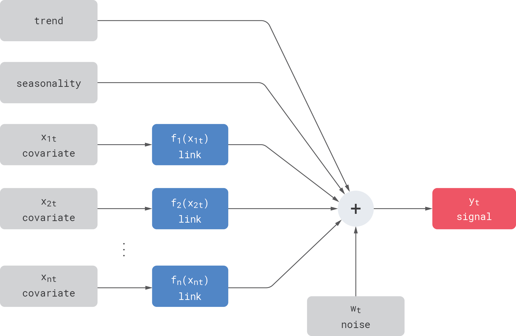
Let us also assume that the signal can be influenced by covariates in some complex way, but we do not know either the shape or the parameters of this dependency. We model this dependency using a link function—we assume that the covariates are directly observed and known, but each of them undergoes some unknown transformation (specified via a link function) before being added into the signal. More concretely, we focus on the following types of link functions:
- Linear link. The covariate is linearly transformed (scaled and shifted) before it is added to the signal. For example, the dependency between the product price (covariate) and demand (signal) is sometimes modeled as linear in applications where changes in price are small.
- Nonlinear link. The covariate undergoes some nonlinear transformation—for example, $\exp(\cdot)$ or $\tanh(\cdot)$—before being added to the signal. In the example with price and demand, the most commonly used price-response models are nonlinear—for example, the constant-elasticity model. Another example is marketing mix modeling, where the marketing spend and outcomes (conversion rates or revenues) typically have nonlinear S-shaped dependency that reflects the principle of diminishing returns.
- Memory link (carryover link). In many cases, the covariate takes effect with a delay or has some long-lasting effect on the signal. In the example with price and demand modeling, it is known that discounts sometimes have a pull-forward effect: consumers buy and stockpile an excessive amount of products under the lower price, and this negatively impacts the future sales after the discount period ends. The same is true for marketing mix modeling, where advertising has carryover effects. One natural way to model this type of a link is the convolution operation: the covariate is convolved with some kernel before being added to the signal.
- Composite link. In some cases, two or more link functions can be chained. For instance, investments into advertising can be prone to nonlinear saturation (diminishing returns) but can also create long-lasting effects on conversions or revenues, so the relationship between the investments and conversions can be modeled as
$$
\text{conversions} = f_m(f_s(\text{investments}))
$$
where $f_s$ is a nonlinear saturation link, and $f_m$ is a memory link.
In most forecasting applications, one has multiple covariates with different link functions. For instance, demand on a certain product can be influenced by the product’s own price, prices of substitutable products (demand cannibalization and halo effects), weather, and so on. In statistics, this structure with multiple active components and nonlinear link functions is known as generalized additive model (GAM).
The following code snippet shows a simple signal generator that implements the above assumptions (the full code is available on GitHub as a part of the TensorHouse project).
Signal Generation. Click to expand the code sample.
def linear_link(x):
    return x

def sigmoid_link(x, scale = 10):
    return 1 / (1 + np.exp(-scale*x))

def mem_link(x, length = 50):
    mfilter = np.exp(np.linspace(-10, 0, length))
    return np.convolve(x, mfilter/np.sum(mfilter), mode='same')

def create_signal(links = [linear_link, sigmoid_link, mem_link]):
    days_year = 365
    quaters_year = 4

    # two years of data, daily resolution
    idx = pd.date_range(start='2018-01-01', end='2020-01-01', freq='D')

    n = len(df.index)
    trend = np.zeros(n)
    seasonality = np.zeros(n)
    for t in range(n):
        trend[t] = 2.0 * t/n
        seasonality[t] = 2.0 * np.sin(np.pi * t/days_year*quaters_year)

    covariates = ... # create several series of length n
    covariate_links = [ links[i](covariates[i]) for i in range(len(covariates)) ]

    noise = np.random.randn(n)

    signal = trend + seasonality + np.sum(covariate_links, axis=0) + noise

    return create_df(idx, signal, trend, seasonality,
                     covariates, covariate_links, noise)
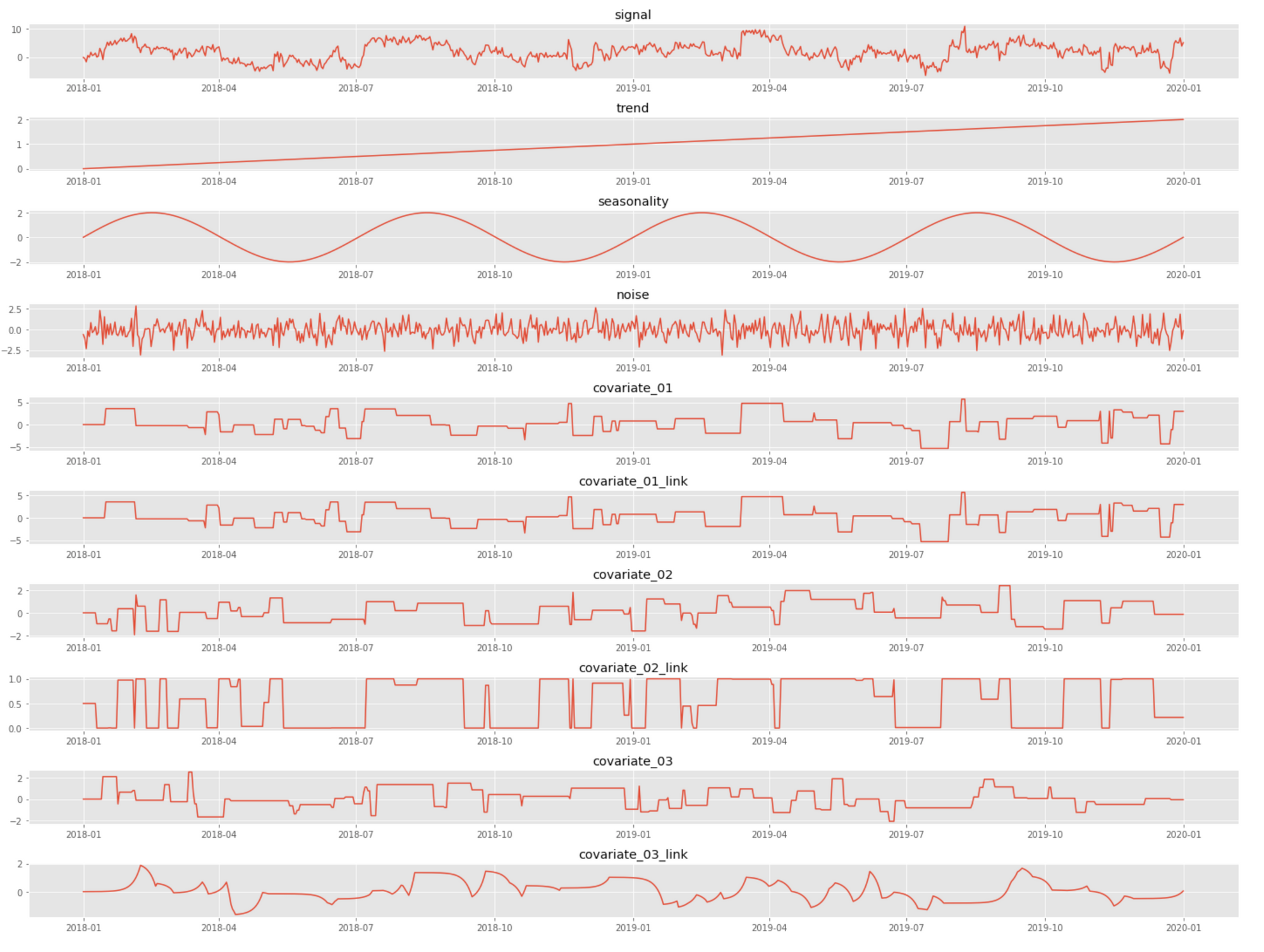
An example realization of the signal and its components produced by the above code is shown in the figure below. Note how the link function stretches covariate 2 in almost a binary function, and covariate 3 is significantly shifted in time (delayed).
Assuming the above setup, we may be interested in researching the following questions:
- How to quantify the contribution of individual covariates into the signal?
- How to estimate (recover) nonlinear link functions?
- How to detect link functions with memory effects and estimate their convolution kernels?
- How to estimate unobserved trend and seasonal components?
All these questions can ultimately be tied to the problem of decomposing the observed signal(s) into hidden components so that each component can be studied in isolation. In addition, we are generally interested in forecasting both observed signals and hidden components and in estimating the distribution (i.e., uncertainty) of the components and forecasts.
The above questions are utterly important in many practical applications. In our running example with price–demand data, a price manager is certainly interested in understanding the shape of link functions (and memory effects in particular), building demand forecasts for different pricing scenarios, and estimating the uncertainty of these forecasts to weigh benefits against risks.
In the remainder of this article, we build several common time series models and explore how to use them for solving the problems stated above. Although some basic capabilities such as forecasting are provided by all models, each model has unique advantages for certain types of analyses.
Analysis Using GBDT
We start with building a gradient boosted decision tree (GBDT) model, which is arguably the most common approach for time series forecasting in enterprise applications. We engineer some basic features that include covariates and lags, split data into train and test sets, fit a model using LightGBM, create a seven days ahead forecast, and visualize it. The implementation is shown in the code snippet below.
LightGBM Model Fitting and Forecasting. Click to expand the code sample.
#
# engineer features for the model
#
def features_regression(df):
    observed_features = ['covariate_01', 'covariate_02', 'covariate_03']
    dff = df[['signal'] + observed_features]

    dff['year'] = dff.index.year
    dff['month'] = dff.index.month
    dff['day_of_year'] = dff.index.dayofyear

    feature_lags = [7, 14, 21, 28, 35, 42, 49, 120, 182, 365]
    for lag in feature_lags:
        dff.loc[:, f'signal_lag_{lag}'] = dff['signal'].shift(periods=lag, fill_value=0).values

    return dff

#
# train-test split
#
def split_train_test(df, train_ratio):
    y_train, y_test = [], []
    x_train, x_test = [], []
    split_t = int(len(df)*train_ratio)

    y = df['signal']
    y_train = y[:split_t]
    y_test = y[split_t:]

    xdf = df.drop('signal', inplace=False, axis=1)
    x_train = xdf[:split_t]
    x_test = xdf[split_t:]

    return x_train, y_train, x_test, y_test

#
# fit LightGBM model
#
def fit_lightgbm(x_train, y_train, x_test, y_test, n_estimators=100):

    model = lightgbm.LGBMRegressor(
        boosting_type = 'gbdt',
        n_estimators=n_estimators)

    model.fit(x_train,
              y_train,
              eval_set=[(x_train, y_train), (x_test, y_test)],
              eval_metric='mape')

    return model

#
# generate data sample and fit the model
#
df = features_regression(create_signal(links = [linear_link, linear_link, mem_link]))
train_ratio = 0.8
x_train, y_train, x_test, y_test = split_train_test(df, train_ratio)
model = fit_lightgbm(x_train, y_train, x_test, y_test)

#
# plot the forecast
#
forecast = model.predict(pd.concat([x_train, x_test]))
fig, ax = plt.subplots(1, figsize=(20, 5))
ax.plot(df.index, forecast, label='Forecast (7 days ahead)')
ax.plot(df.index, df['signal'], label='Actuals')
ax.axvline(x=df.index[int(len(df) * train_ratio)], linestyle='--')
ax.legend()
An example plot produced by the above implementation with the actual signal vs. forecast is shown below.

We are now all set to perform some of the tasks defined in the introduction section. Let us start with estimating the uncertainty of the forecast.
Forecast Distribution
The GBDT model we just developed uses the mean squared error (MSE) loss function and thus estimates the conditional mean of the response variable across values of the covariates. This is a useful but incomplete result because we generally want to estimate not only the mean but also the distribution of the response variable or, at least, some properties related to this distribution such as confidence intervals. This problem can be approached in several different ways, and we examine two of them in this section.
The first technique we examine is quantile regression that allows us to estimate arbitrary quantiles of the forecast [1]. In practice, it is often enough to estimate specific quantiles (e.g., 95th percentile), but we can approximate the full forecast distribution through estimating multiple quantiles (e.g., 5th, 10th, ..., 95th). One of the main benefits of quantile regression is that it can be implemented by tweaking the loss function; thus, it can be applied on top of most ML frameworks, including LightGBM and XGBoost.
Let us briefly review the theory behind quantile regression. Recall that the least squares regression estimates the mean of the response variable by solving the following optimization problem:
$$
\min_{\mu} \mathbb{E}[\ (y - \mu)^2 \ ]
$$
where $y$ is the response variable, and $\mu$ can be a constant or a function of the covariates. It can also be shown (and we will do so in a moment) that minimization of the absolute error instead of the squared error produces the median estimate.
$$
\min_{m} \mathbb{E}[\ |y - m| \ ]
$$
Quantile regression extends this result to the estimation of the $\tau$th quantile of the response variable, which is defined as follows:
$$
q(\tau) = \text{inf}[\ y\ |\ F(y) \ge \tau\ ] = F^{-1}(\tau)
$$
where $F(y)$ is the cumulative distribution function of the response variable. Let us show that the quantile can be estimated by solving the following problem:
$$
\min_{q} \mathbb{E}[\ \rho_\tau(y - q) \ ]
$$
where $\rho_\tau$ is the asymmetric version of the absolute value function.
$$
\rho_\tau(x) = \begin{cases}
(\tau-1)x,\quad &x<0\\
\tau x,\quad &x\ge0
\end{cases}
$$
To prove the above statement, we can solve the optimization problem by differentiating the expectation term with regard to $q$ and equating the derivative to zero:
$$
\begin{aligned}
\mathbb{E}[ \rho_\tau(y-q) ] &= \int_{-\infty}^{\infty} \frac{d\rho_\tau(y-q)}{dq}p(y)dy \\
&= (\tau-1) \int_{-\infty}^{q} p(y)dy + \tau \int_{q}^{\infty} p(y)dy \\
&= (\tau-1)F(q) + \tau(1-F(q)) = 0
\end{aligned}
$$
where $p(y)$ is the probability density function of the response variable. The last line implies that
$$
\tau = F(q)
$$
and, consequently, that $q = F^{-1}(\tau)$, which is the definition of the $\tau$th quantile introduced earlier. Note that $\rho_\tau$ reduces to the absolute value function in case of $\tau=0.5$, and this corresponds to the median estimate mentioned earlier. The relationship between the three loss functions becomes apparent when we plot them side by side:

The implementation of quantile regression with LightGBM is shown in the code snippet below. It is very straightforward (we just change the loss function), but we need to fit a separate model for each percentile.
Quantile Regression Using LightGBM. Click to expand the code sample.
#
# fit the quantile regression model with LightGBM
#
def fit_lightgbm_quantile(x_train, y_train, x_test, y_test, alpha, n_estimators=100):

    model = lightgbm.LGBMRegressor(
        boosting_type = 'gbdt',
        objective = 'quantile',        # quantile loss function
        alpha = alpha,
        n_estimators=n_estimators)

    model.fit(x_train,
              y_train,
              eval_set=[(x_train, y_train), (x_test, y_test)],
              eval_metric='mape')

    return model

#
# generate data sample and fit models
#
df = features_regression(create_signal(links = [linear_link, linear_link, mem_link]))
train_ratio = 0.8
x_train, y_train, x_test, y_test = split_train_test(df, train_ratio)
alphas = [0.90, 0.80, 0.70, 0.60]
model_mean = fit_lightgbm(x_train, y_train, x_test, y_test)
models_upper = [fit_lightgbm_quantile(x_train, y_train, x_test, y_test, 1 - alpha)
                for alpha in alphas]
models_lower = [fit_lightgbm_quantile(x_train, y_train, x_test, y_test, alpha)
                for alpha in alphas]

#
# plot the forecasts
#
x = pd.concat([x_train, x_test])
forecasts_upper = [model.predict(x) for model in models_upper]
forecasts_lower = [model.predict(x) for model in models_lower]
forecast_mean = model_mean.predict(x)
...
The confidence intervals estimated using this technique are visualized in the following plot:

The alternative to quantile regression is to assume a parametric distribution for the forecast samples and estimate its parameters. For instance, we can assume that the forecast values are normally distributed and estimate both mean and variance for each time step. This idea was developed in [2] and further implemented in the NGBoost library, where distribution parameters are estimated using GBDTs. The code snippet below shows how to fit the NGBoost model, estimate the distribution parameters, and visualize quantiles computed based on the distribution function.
Forecast Distribution Estimation Using NGBoost. Click to expand the code sample.
from ngboost import NGBRegressor
from scipy.stats import norm

ngb = NGBRegressor().fit(x_train, y_train)   # Normal distribution by default
y_preds = ngb.predict(x)
y_dists = ngb.pred_dist(x)

fig, ax = plt.subplots(1, figsize=(20, 5))
alphas = [0.99, 0.90, 0.80, 0.70]
for i, alpha in enumerate(alphas):
    rng = norm(loc=0.0, scale=y_dists.params['scale']).ppf(alpha)
    ax.fill_between(df.index, y_preds + rng, y_preds - rng,
                    alpha=0.5, ec='None', label=f'Forecast CI ({alpha})')
ax.plot(df.index, df['signal'], color='r', alpha=0.2, label='Actuals')
ax.plot(df.index, y_preds, color='k', alpha=0.5, label='Forecast mean')
This produces a result similar to that of quantile regression:

Assessing the uncertainty of the forecasts produced by GBDT models is an important topic because of the widespread use of GBDT in enterprise applications, and both quantile regression and NGBoost are useful tools for addressing this problem. However, Bayesian methods can address this problem in a more comprehensive and consistent way, so we get back to this topic in one of the following sections.
Contribution of Individual Covariates
Another task is to analyze how individual covariates influence the signal. This problem can also be approached in several different ways, with Shapley values being one of the most commonly used and well-known methods. The idea behind Shapley values is to measure the contribution of individual features into the response variable by comparing model predictions for inputs with this feature present against model predictions for inputs with this feature withheld [3]. This approach is generally applicable to any (black-box) model and allows for computing feature contributions at individual input points (time steps in the case of time series). More concretely, we define the Shapley value for feature $x_i$ given input vector $x$ as follows:
$$
\phi(x_i, x) = \sum_{z \subseteq x} w_z\cdot ( f(z) - f(z_{-i}) )
$$
where $z$ runs over all possible subsets of $x$ ($z$ is a copy of $x$ with some positions zeroed out), $f(\cdot)$ is the model, $z_{-i}$ is $z$ with the $i$th feature zeroed out, and $w_z$ is a weight computed based on the number of non-zeroed positions in $z$.
The exact computation of Shapley values can be computationally challenging, but there exist good approximations. One of the most common choices is SHAP [4]. The code snippet below shows how SHAP values can be estimated and visualized for the LightGBM model we built in the previous section.
Covariate Contribution Analysis Using SHAP. Click to expand the code sample.
import shap

series_to_explain = pd.concat([x_train, x_test])
explainer = shap.TreeExplainer(model)
shap_values = explainer.shap_values(series_to_explain)

feature_names=['covariate_01', 'covariate_02', 'covariate_03']
cols = [series_to_explain.columns.get_loc(c) for c in feature_names]
values = shap_values[:, cols]
fig, ax = plt.subplots(2, figsize=(20, 6))
for i in [0, 1]:
    ax[i].stackplot(series_to_explain.index, values.T,
                    alpha=0.8, labels=feature_names)
    ax[i].plot(series_to_explain.index, series_to_explain[f'covariate_0{i+1}'],
               color='k', label=f'covariate_0{i+1}')
    ax[i].legend()
The above implementation produces the following result for the first two covariates:

The above plot shows a clear correlation between covariate values (black line) and their contributions into the signal. The first covariate has the largest magnitude and thus its effect is the most pronounced; the second covariate adds a relatively thin layer on top of the first one.
Link Function Shape
The analysis in the previous section estimates the magnitude of the covariate contributions, but it does not exactly show how the signal depends on its covariates. In other words, it does not estimate the shape of the link function. Link function estimates are important in many applications where the covariate values are the subjects of optimization. For instance, a price manager who analyzes the dependency between price and demand needs to exactly know how the demand depends on a price and where the steep and flat zones are located. The same is the case for predictive maintenance, where one might be looking for the optimal usage intensity, fuel levels, and so on.
This problem can be addressed using partial dependence plots (PDP). This technique is similar to Shapley values in that it analyzes the marginal effect an isolated feature has on the response variable. More formally, we define the partial dependence function for feature $x_i$ as follows:
$$
\psi(x_i) = \mathbb{E}_ {x_i}[ f(x_ {-i}, x_i) ]
$$
where $x_{-i}$ is the input vector with the feature $x_i$ being removed or zeroed out, and $f(\cdot)$ is the model. The partial dependence function defined above can be estimated by averaging the predictions for all data samples for each value of $x_i$. The implementation of the PDP analysis and example results are shown below.
Partial Dependence Plots. Click to expand the code sample.
from pdpbox import pdp

df = features_regression(create_signal(links = [linear_link, sigmoid_link, mem_link]))
train_ratio = 0.8
x_train, y_train, x_test, y_test = split_train_test(df, train_ratio)
model = fit_lightgbm(x_train, y_train, x_test, y_test)

for i in [1, 2]:
    pdp_isolate = pdp.pdp_isolate(
        model=model,
        dataset=series_to_explain,
        model_features=series_to_explain.columns,
        feature=f'covariate_0{i}',
        num_grid_points=20)
    pdp.pdp_plot(pdp_isolate, f'covariate_0{i}', plot_lines=True, frac_to_plot=100)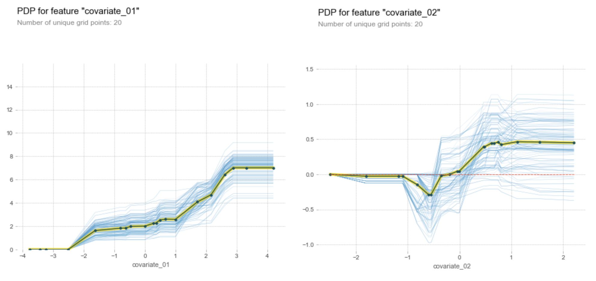
We can see that PDP provides reasonably good estimates for the link functions: the link function for the first covariate is approximately linear except the outliers at the upper and lower ends, and the link function for the second covariate is clearly a sigmoid function.
Memory Effects
The last problem we research using the GBDT model is the analysis of the memory effects. Our goal is to estimate link functions that potentially blend multiple samples (lags) of the covariate. The straightforward solution for this problem is lagged regression that uses shifted copies of the covariate as additional input features and estimates their contributions. For example, we can specify the linear lagged regression model as follows:
$$
y_t = \sum_{i=0}^{m} \beta_{i} x_{t-i}
$$
where $x_t$ is the covariate, $y_t$ is the response variable, and $\beta$ are the regression coefficients. This approach can be applied to nonlinear models, but one needs to combine it with a feature significance measure because regression coefficients are not explicitly available.
The code snippet below shows how the lagged regression idea, LightGBM, and Shapley values are combined to estimate the convolutional link function:
Lagged Regression Using LightGBM and SHAP. Click to expand the code sample.
#
# prepare features for lagged regression
#
df_original = create_signal()
observed_features = ['covariate_01', 'covariate_02']
df = df_original[['signal'] + observed_features]
df['year'] = df.index.year
df['month'] = df.index.month
df['day_of_year'] = df.index.dayofyear
lags = np.arange(0, 50, 5)
for lag in lags:
    df.loc[:, f'covariate_03_lag_{lag}'] =
    df_original['covariate_03'].shift(periods=lag, fill_value=0).values

#
# LightGBM
#
x_train, y_train, x_test, y_test = split_train_test(df, train_ratio)
model = fit_lightgbm(x_train, y_train, x_test, y_test)

#
# SHAP
#
series_to_explain = pd.concat([x_train, x_test])
patch_model(model)
explainer = shap.TreeExplainer(model)
shap_values = explainer.shap_values(series_to_explain)

#
#
#
feature_names=[f'covariate_03_lag_{lag}' for lag in lags]
cols = [series_to_explain.columns.get_loc(c) for c in feature_names]
values = shap_values[:, cols]
fig, ax = plt.subplots(1, figsize=(20, 5))
ax.stackplot(series_to_explain.index, values.T, alpha=0.8)
ax.plot(series_to_explain.index, df_original['covariate_03_link'],
        color='k', label='True covariate link')
plt.legend()
plt.show()
This implementation produces the following results that demonstrate a reasonably accurate estimate of the true convolutional link:

This approach, however, is not particularly stable in the case of complex randomized models such as GBDT, and one needs to carefully tune the input feature set and model capacity to obtain reliable results. This problem can be mitigated using a simpler (e.g., linear) model or submodel or using other regularizations, as we discuss later in the section on Bayesian methods.
Analysis Using LSTM
The second group of methods we consider is based on recurrent neural networks (RNNs). In the context of this article, RNNs have several unique advantages. First, RNNs provide a powerful toolkit for time series forecasting that is being increasingly used in enterprise applications. Second, RNNs play a central role in natural language processing (NLP), and a broad range of interpretability-related techniques and extensions has been developed in connection to NLP problems over the last several years.
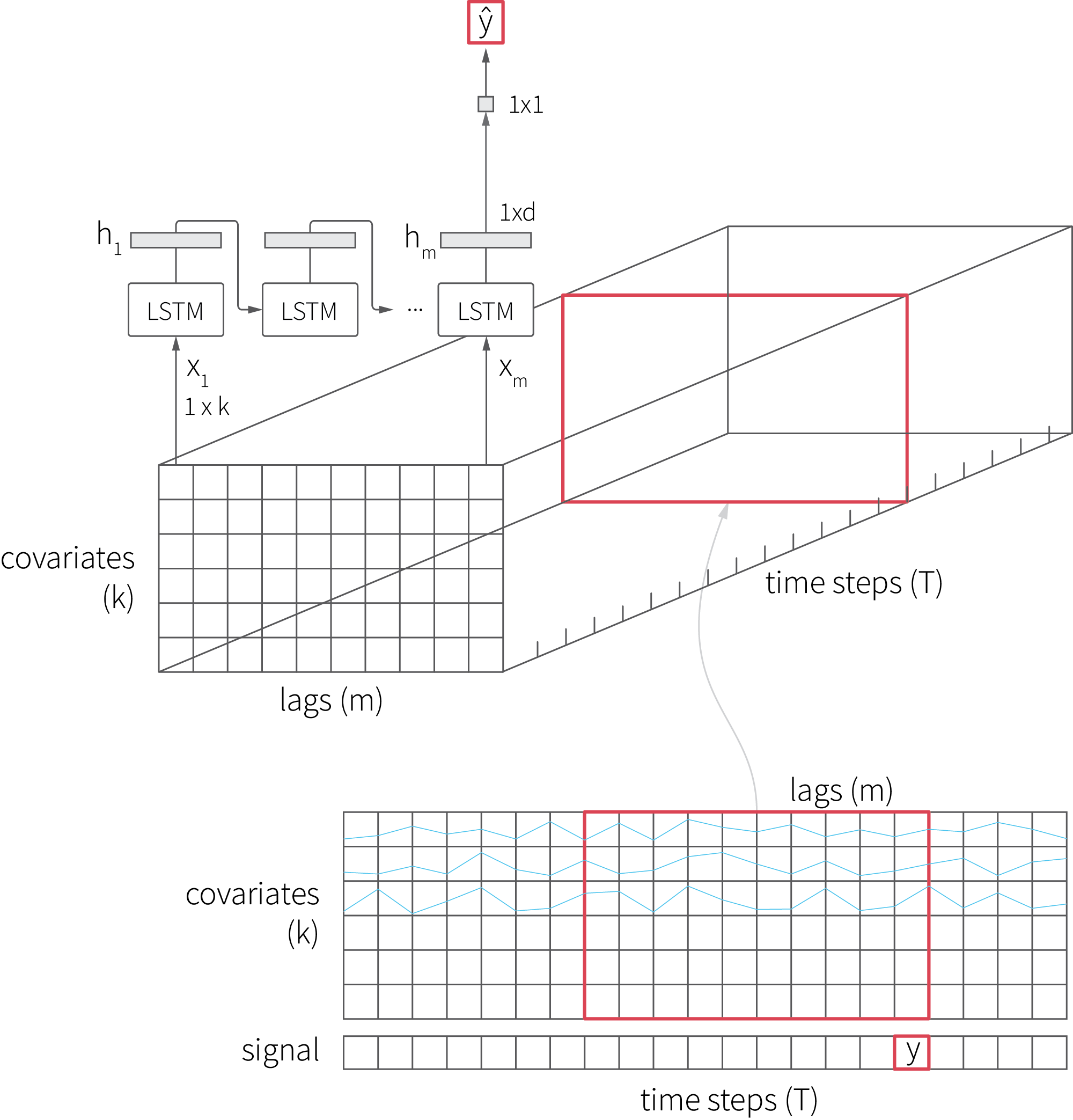
We start with implementing the basic LSTM model using Keras and fitting it on a signal with two covariates. Note that the shape of the input is very different from that of the input we used for the LightGBM model because LSTM consumes a batch of feature vectors for each time step, so the input is a three-dimensional tensor, as shown in the figure below:
The implementation code is provided below.
Basic LSTM Model Using Keras. Click to expand the code sample.
#
# engineer features and create input tensors
#
def prepare_features_rnn(df):
    df_rnn = df[['signal', 'covariate_01', 'covariate_02']]
    df_rnn['year'] = df_rnn.index.year
    df_rnn['month'] = df_rnn.index.month
    df_rnn['day_of_year'] = df_rnn.index.dayofyear

    def normalize(df):    # input normalization is essential for RNNs
        x = df.values
        min_max_scaler = preprocessing.MinMaxScaler()
        x_scaled = min_max_scaler.fit_transform(x)
        return pd.DataFrame(x_scaled, index=df.index, columns=df.columns)

    return normalize(df_rnn)

#
# train-test split and adjustments
#
def train_test_split(df, train_ratio, forecast_days_ahead, n_time_steps, time_step_interval):
    # length of the input time window for each sample
    # i.e., the offset of the oldest sample in the input
    input_window_size = n_time_steps*time_step_interval

    split_t = int(len(df)*train_ratio)
    x_train, y_train = [], []
    x_test, y_test = [], []
    y_col_idx = list(df.columns).index('signal')
    for i in range(input_window_size, len(df)):
        t_start = df.index[i - input_window_size]
        t_end = df.index[i]

        # we zero out last forecast_days_ahead signal observations,
        # but covariates are assumed to be known for all time steps
        x_t = df[t_start:t_end:time_step_interval].values.copy()
        if time_step_interval <= forecast_days_ahead:
            x_t[-int((forecast_days_ahead) / time_step_interval):, y_col_idx] = 0

        y_t = df.iloc[i]['signal']

        if i < split_t:
            x_train.append(x_t)
            y_train.append(y_t)
        else:
            x_test.append(x_t)
            y_test.append(y_t)

    return np.stack(x_train), np.hstack(y_train), np.stack(x_test), np.hstack(y_test)

#
# parameters
#
n_time_steps = 40         # length of LSTM input in samples
time_step_interval = 2    # sampling interval, days
hidden_units = 8          # LSTM state dimensionality
forecast_days_ahead = 7
train_ratio = 0.8

#
# generate data and fit the model
#
df = create_signal()
df_rnn = prepare_features_rnn(df)
x_train, y_train, x_test, y_test = train_test_split(df_rnn, train_ratio, forecast_days_ahead, n_time_steps, time_step_interval)

n_samples = x_train.shape[0]
n_features = x_train.shape[2]

input_model = Input(shape=(n_time_steps, n_features))
# we configure the model to return a sequence of states
# to enable detailed analysis
lstm_state_seq, state_h, state_c = LSTM(hidden_units,
                                        return_sequences=True,
                                        return_state=True)(input_model)
output_dense = Dense(1)(state_c)
model_lstm = Model(inputs=input_model, outputs=output_dense)

model_lstm.compile(loss='mean_squared_error',
                   metrics=['mean_absolute_percentage_error'],
                   optimizer='RMSprop')
model_lstm.fit(x_train, y_train, epochs=20, batch_size=4,
               validation_data=(x_test, y_test), use_multiprocessing=True)
Although LSTM is a complex model with a large number of parameters, there exist good tools for its introspection. One option is to use black-box interpretation methods such as Shapley values that we previously discussed in connection with GBDT. Another option is to analyze how the internal state of the model evolves over time. This approach can be insightful because the state vector is a low-dimensional representation of the input samples that tends to align itself with the persistent patterns in the data, resembling principal component analysis.
We implement state tracing in the code snippet below. It visualizes the forecast, internal state evolution, and covariates in one set of plots; therefore, we can assess the dependencies between all these time series. Note that we choose the dimensionality of the hidden state to be sufficiently small (8 units) for producing well-defined components (harmonics).
LSTM State Visualization. Click to expand the code sample.
input_window_size = n_time_steps*time_step_interval
x = np.vstack([x_train, x_test])
y_hat = model_lstm.predict(x)
forecast = np.append(np.zeros(input_window_size), y_hat)

#
# plot the forecast
#
fig, ax = plt.subplots(1, figsize=(20, 5))
ax.plot(df_rnn.index, forecast, label=f'Forecast ({forecast_days_ahead} days ahead)')
ax.plot(df_rnn.index, df_rnn['signal'], label='Signal')
ax.axvline(x=df.index[int(len(df) * train_ratio)], linestyle='--')
ax.legend()
plt.show()

#
# plot the evolution of the LSTM state
#
lstm_state_tap = Model(model_lstm.input, lstm_state_seq)
lstm_state_trace = lstm_state_tap.predict(x)

state_series = lstm_state_trace[:, -1, :].T
fig, ax = plt.subplots(len(state_series), figsize=(20, 15))
for i, state in enumerate(state_series):
    ax[i].plot(df_rnn.index[:len(state)], state, label=f'State dimension {i}')
    for j in [1, 2]:
        ax[i].plot(df_rnn.index[:len(state)],
                   df_rnn[f'covariate_0{j}'][:len(state)],
                   label=f'Covariate 0{j}')

    ax[i].legend(loc='upper right')
plt.show()
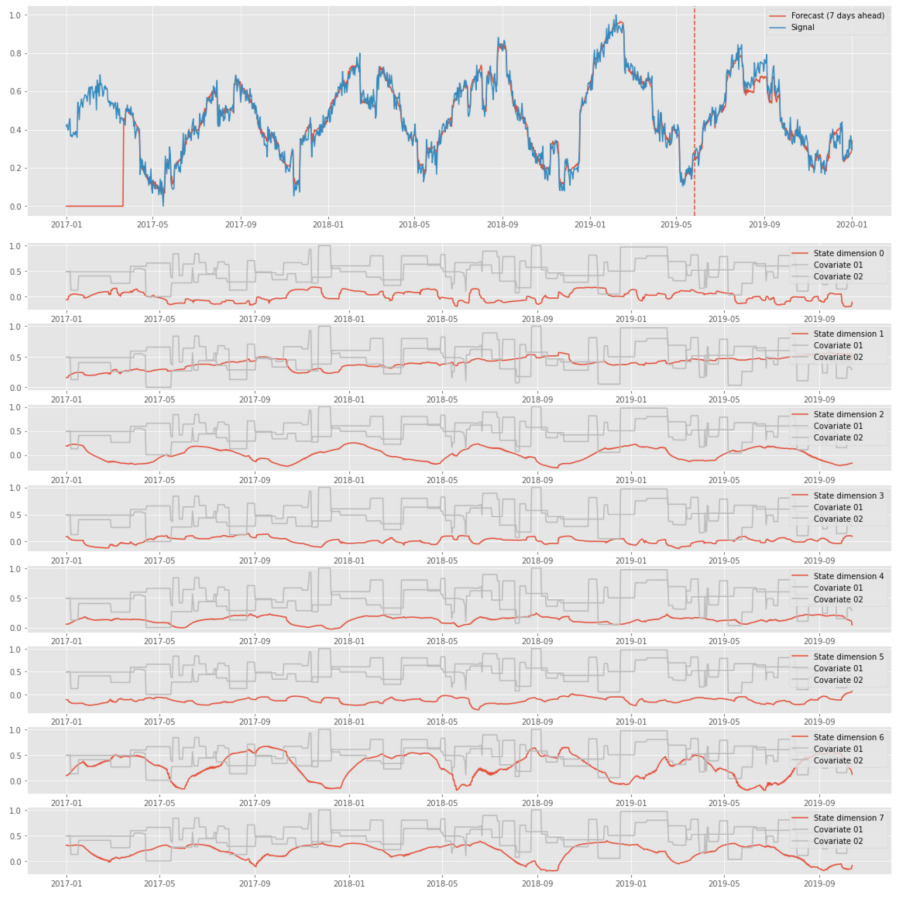
The above plots show that LSTM can perform signal decomposition in an unsupervised way. For instance, state dimension 1 captures the trend, and dimensions 2 and 6 capture seasonality. This decomposition is not particularly useful for the tasks we focus on because of its instability, but it can be useful in some related applications. For instance, one can perform similar analysis for a series of clickstream events and use the dynamics of the hidden state to tell whether a customer is moving toward purchasing, account cancellation, etc. [6].
Memory Effects and LSTMograms
Unlike models that consume aggregated features, LSTM accounts for the order of input samples, but it does not provide a simple way to estimate the contributions of each of these samples. This shortcoming can be addressed using the attention mechanism that adds a layer on top of LSTM cells so that the final output is estimated as a weighted sum of cell outputs, as shown in the figure below:
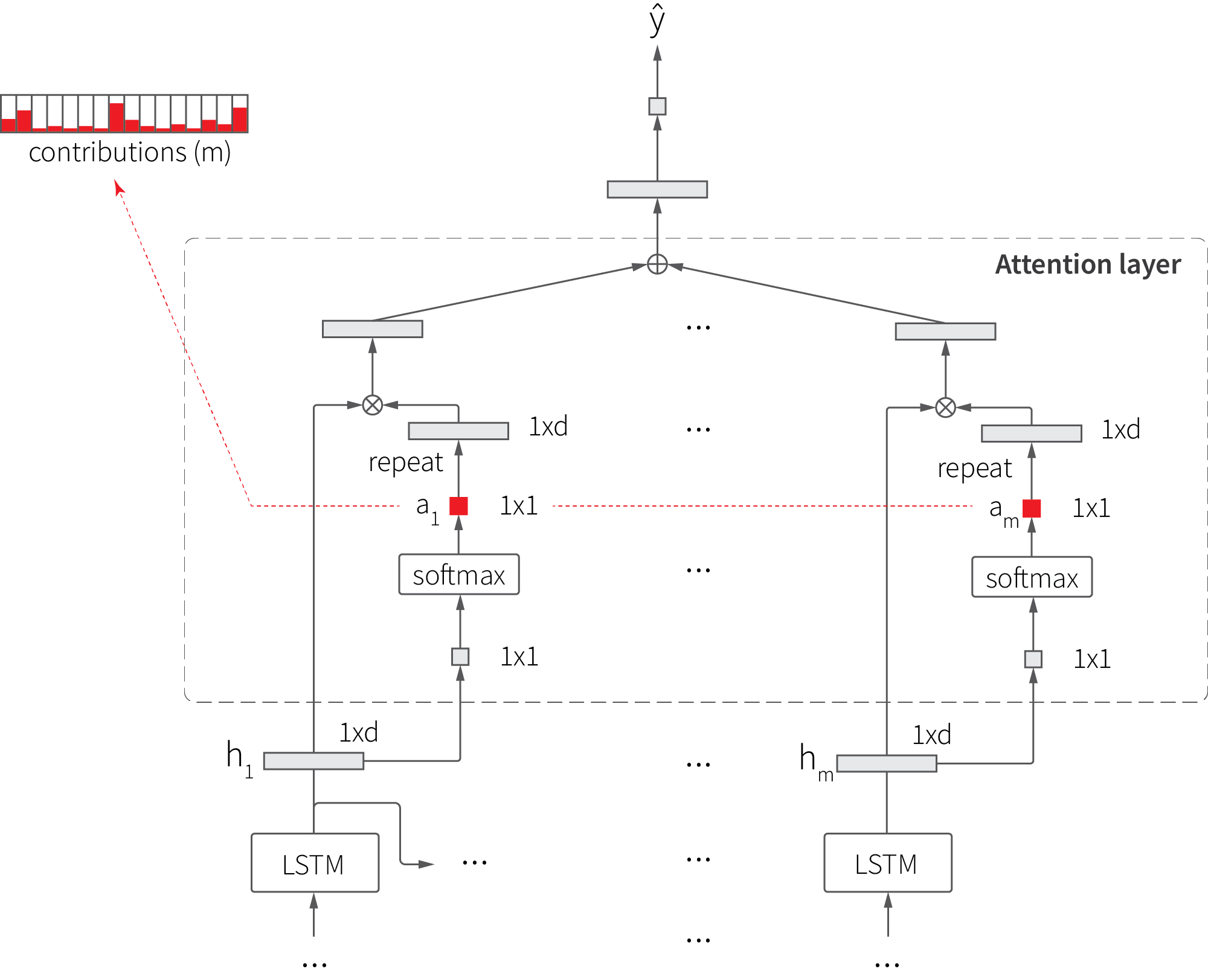
The attention mechanism extends the basic LSTM in two ways. First, an additional layer that maps each hidden state $h$ to weight coefficient $a$ is added, and then the hidden state is multiplied (weighted) by this coefficient. Second, the output is produced based on the weighted sum of hidden states, not just on the last state. This extension generally improves the accuracy of the model, but we are mainly interested in its side effects—the ability to estimate sample contributions using attention weights. This can be particularly useful for the analysis of memory effects.
We start with specifying the LSTM with attention model, as shown in the code snippet below. The implementation of the attention layer closely follows the above diagram.
LSTM With Attention: Model Specification. Click to expand the code sample.
#
# parameters
#
n_time_steps = 5           # length of LSTM input in samples
time_step_interval = 10    # sampling interval, days
hidden_units = 256         # LSTM state dimensionality
forecast_days_ahead = 14
train_ratio = 0.8

def fit_lstm_a(df):
    df_rnn = prepare_features_rnn(df)

    x_train, y_train, x_test, y_test = train_test_split(df_rnn, train_ratio,
                                                        forecast_days_ahead,
                                                        n_time_steps,
                                                        time_step_interval)

    n_steps = x_train.shape[0]
    n_features = x_train.shape[2]

    #
    # define the model: LSTM with attention
    #
    main_input = Input(shape=(n_steps, n_features))
    activations = LSTM(hidden_units, recurrent_dropout=0.1,
                       return_sequences=True)(main_input)

    attention = Dense(1, activation='tanh')(activations)
    attention = Flatten()(attention)
    attention = Activation('softmax', name = 'attention_weigths')(attention)
    attention = RepeatVector(hidden_units * 1)(attention)
    attention = Permute([2, 1])(attention)

    weighted_activations = Multiply()([activations, attention])
    weighted_activations = Lambda(lambda xin: K.sum(xin, axis=-2),
                                  output_shape=(hidden_units,))(weighted_activations)

    main_output = Dense(1, activation='sigmoid')(weighted_activations)

    model_attn = Model(inputs=main_input, outputs=main_output)

    #
    # fit the model
    #
    model_attn.compile(optimizer='rmsprop', loss='mean_squared_error',
                       metrics=['mean_absolute_percentage_error'])
    history = model_attn.fit(x_train, y_train, batch_size=4,
                             epochs=30, validation_data=(x_test, y_test))
    score = model_attn.evaluate(x_test, y_test, verbose=0)

    return model_attn, df_rnn, x_train, x_test
The model consumes sequences of five samples (lags), so the attention layer produces five weights for each input tensor. Consequently, we can feed an input of $T$ time steps into the model and produce a $5 \times T$ matrix of attention weights, where each element $w_{i=1:5,\ t=1:T}$ characterizes the contribution of the lag $i$ into the forecast for time step $t$. This matrix is somewhat similar to spectrograms and scalograms, so we call it LSTMogram here.
To illustrate how LSTMograms work, we generate a pair of datasets (with and without memory-linked covariate), fit the mode for each of them, and visualize the matrix of attention weights. We repeat the process four times to make sure that the results are consistent:
LSTMograms. Click to expand the code sample.
n_evaluations = 4
fig, ax = plt.subplots(n_evaluations, 2, figsize=(16, n_evaluations * 2))
for j, link in enumerate([linear_link, mem_link]):
    for i in range(n_evaluations):
        df = create_signal(links = [link, link])
        model_attn, df_rnn, x_train, _ = fit_lstm_a(df)

        attention_model = Model(inputs=model_attn.input,
                                outputs=model_attn.get_layer('attention_weigths').output)
        a = attention_model.predict(x_train)
        ax[i, j].imshow(a.T, cmap='viridis', interpolation='nearest', aspect='auto')
        ax[i, j].grid(None)
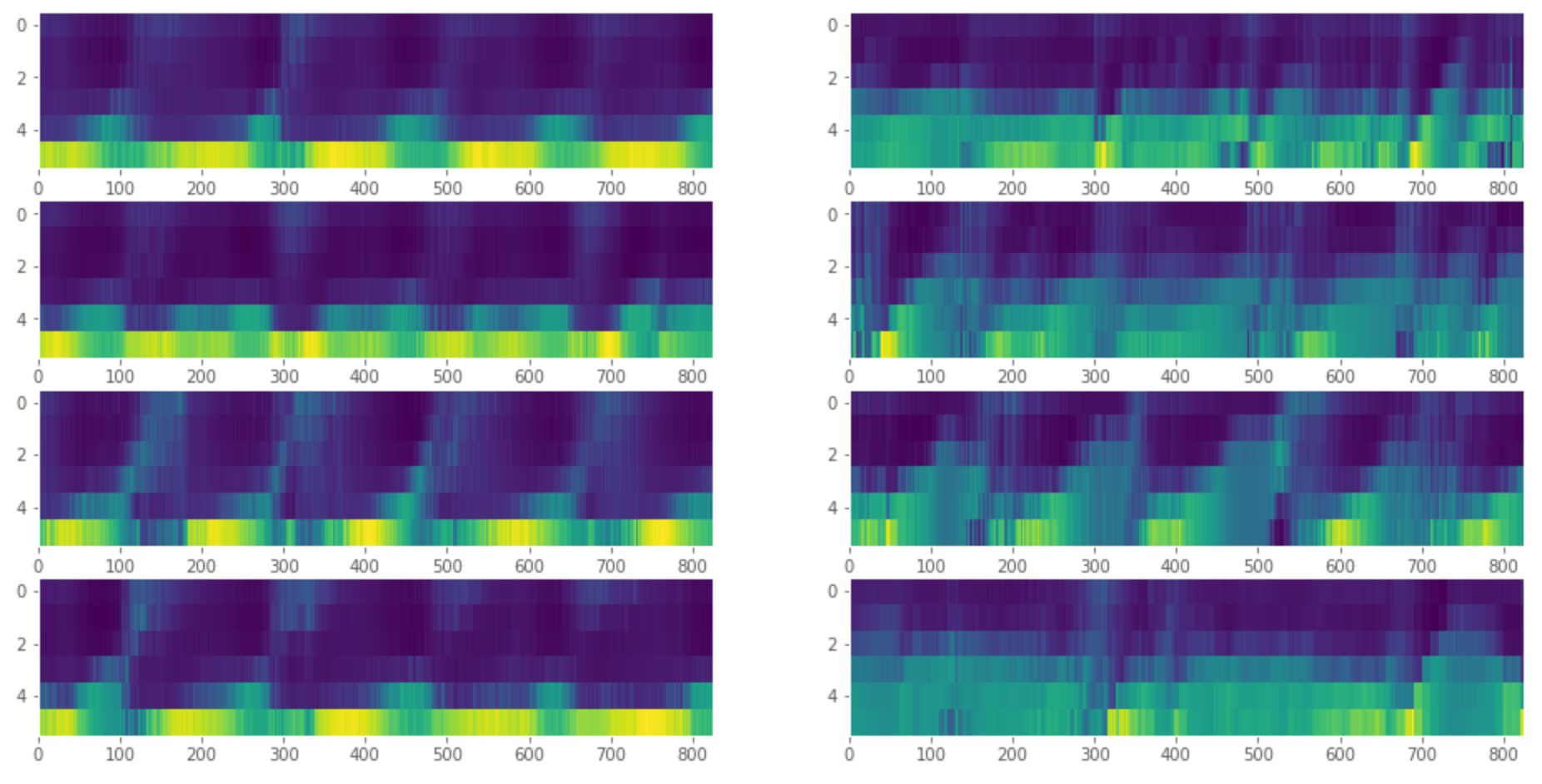
Each of the above heatmaps corresponds to one dataset. The datasets without memory effects are shown on the left, and datasets with memory effects are shown on the right. It is clearly visible that the forecast is mainly influenced by just one lag when the memory effects are absent and by multiple lags when the memory effects are present; thus, the heatmaps on the right-hand side are much more "blurry" than the ones on the left-hand side.
Analysis Using VAR
The next tool we consider is the vector autoregressive (VAR) model. From the forecasting perspective, VAR is a linear low-capacity model that is not particularly suitable for many enterprise use cases. However, it provides unique capabilities for memory effects analysis that are worth a discussion.
The VAR model considers the case of several interrelated time series. Assuming that we observe $n$ time series $y_{it}$, the $p$th order VAR model of dimension $n$ is defined as follows:
$$
\mathbf{y}_ t = \mathbf{c} + \sum_{i=1}^p \mathbf{A}_ i \mathbf{y}_ {t-i} + \mathbf{u}_ t
$$
where $\mathbf{c}$ is $1\times n$ vector of constants, $\mathbf{A}_i$ is a set of $n\times n$ matrices of regression coefficients, and $\mathbf{u}_t$ is a $1\times n$ zero mean noise. For instance, the VAR(1) model for two time series and one time lag is specified as follows.
$$
\begin{aligned}
y_{1,t} &= c_{1} + a_{11,1}y_{1,t-1} + a_{12,1}y_{2,t-1} + u_{1,t} \\
y_{2,t} &= c_{2} + a_{21,1}y_{1,t-1} + a_{22,1}y_{2,t-1} + u_{2,t}
\end{aligned}
$$
An important property of the VAR model is its ability to estimate how one variable $y_r$ responds to a unit impulse in another variable $y_s$. More specifically, the model estimates the impulse response function (IRF) that shows how $y_r$ oscillates over a certain period of time in response to a unit change in $y_s$. For example, a single change in price can make the demand oscillate for some period of time until it stabilizes at a new level; we are interested in estimating the shape of this oscillation.
To see how VAR can be used to estimate the IRF, let us write the model in a lag operator form:
$$
\mathbf{A}(B)\mathbf{y}_t = \mathbf{u}_t
$$
where $B$ is the lag operator and $\mathbf{A}$ is the lag polynomial in $B$.
$$
\mathbf{A}(B) = \mathbf{I}_n - \mathbf{A}_1B - \ldots - \mathbf{A}_p B^p
$$
Consequently, we can define the vector moving average representation as
$$
\mathbf{y}_ t = \mathbf{A}^{-1}(B)\mathbf{u}_ t = \mathbf{\Psi}(B)\mathbf{u}_ t = \mathbf{u}_ t + \sum_{i=1}^\infty \mathbf{\Psi}_ i \mathbf{u}_ {t-i}
$$
where
$$
\begin{aligned}
\mathbf{\Psi}_ i &= \sum_{j=1}^i \mathbf{A}_ j \mathbf{\Psi}_ {i-j} \quad \\
\mathbf{\Psi}_ 0 &= \mathbf{I}_ n \\
\mathbf{\Psi}_ i &= \mathbf{0} \quad i<0
\end{aligned}
$$
Conceptually, the response of $y_r$ to a unit shock in $y_s$ is given by the IRF specified by the sequence $\phi_{rs,1}, \psi_{rs, 2}, \ldots$, where $\psi_{rs,i}$ is the $(r,s)$th element of the matrix $\mathbf{\Psi}_i$. The canonical procedure for impulse response analysis also includes the renormalization of matrices $\mathbf{\Psi}$ to remove the effects of potential correlations in noise sample $u_t$, but we omit these details here because we are only discussing the concept.
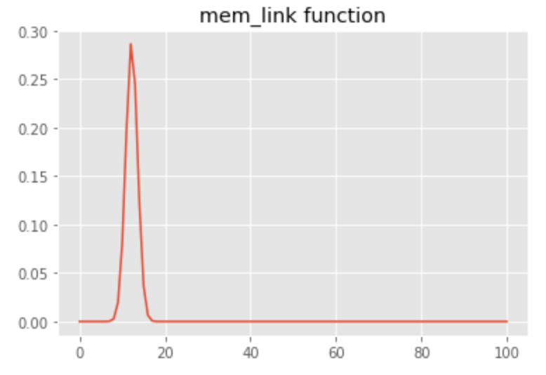
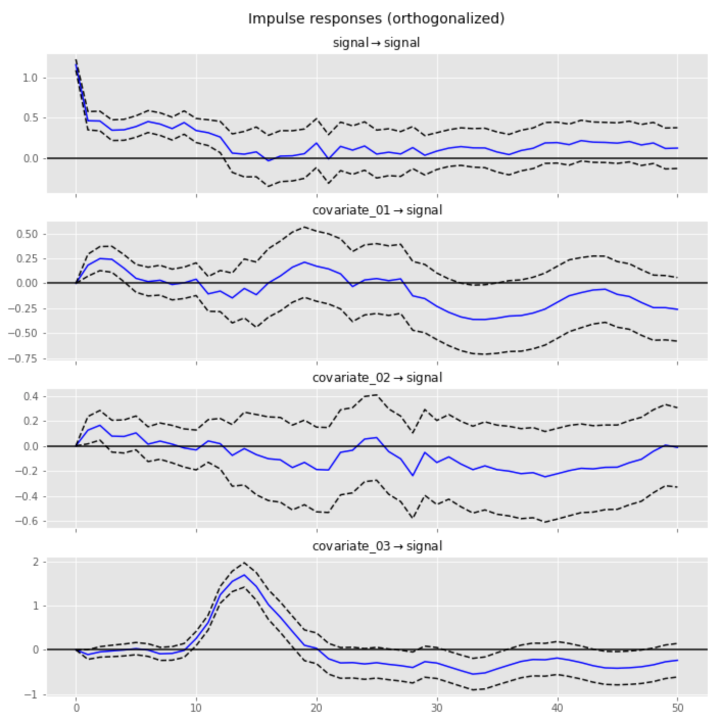
We illustrate the above concept using a signal that includes three covariates with linear, sigmoid, and convolutional links, respectively. We use a bell-shaped filter for the convolutional link that is equivalent to a 15-sample delay with subtle blurring of the original covariate:
The following plot shows an example of the original series and its transformation using the link function we have defined:

Next, we fit the VAR model using the statsmodels library and visualize the IRF of the signal for each covariate. The implementation is provided in the code snippet below.
Impulse Response Analysis Using VAR. Click to expand the code sample.
df = create_signal()

#
# subtract the rolling mean to remove trend/seasonality
#
df['signal'] = df['signal'] - df['signal'].rolling(int(len(df)/16)).mean()
df[np.isnan(df)] = 0

#
# fit the VAR model
#
endog_cols = ['signal', 'covariate_01', 'covariate_02', 'covariate_03']
df_endog = df[endog_cols]

split_t = int(len(df_endog) * 0.8)
idx_train, idx_test = df_endog.index[:split_t], df_endog.index[split_t:]
x_endog_train, x_endog_test = df_endog[:split_t], df_endog[split_t:]
model_var = VAR(endog = x_endog_train, dates = idx_train, freq = 'D')
model_var_fitted = model_var.fit(30, trend='c')

irf = model_var_fitted.irf(50)
irf.plot(orth=True, response='signal')
The resulting IRF for the third covariate quite closely reproduces the filter in terms of both shape and position of the peak (15-sample offset), whereas the IRFs for the other two covariates have much lower magnitudes and do not indicate the presence of memory effects:
Analysis Using Bayesian Methods
The methods we have examined thus far help to analyze certain effects such as saturation or carryover, but none of them provides a sufficiently expressive and generic framework that can be applied to a broad range of signals with complex internal structure. In this section, we discuss how this gap can be closed using Bayesian methods.
In Bayesian analysis, we specify the distribution of the observed data as some function that reflects our assumptions about the internal structure of the process that generated these data; then we use numerical methods to estimate the distributions of the model parameters. In this way, we can explicitly specify transformations such as saturation, carryover, or any composition of those and estimate the parameters of the corresponding link functions. It is also important that we can specify prior distributions of the model parameters to incorporate additional assumptions or known facts. We demonstrate these capabilities in the example below without going deeply into the theoretical details.
Let us consider the case of a composite link where each covariate is presumably transformed using a sigmoid function and then convolved with the exponential decay filter:
$$
\begin{aligned}
y_t &= \alpha_0 + \sum_i \alpha_i \sum_{q=0}^n k_i^t \cdot s_i(x_{i,\ t-q})\\
s_i(x) &= \frac{1}{1 + \exp(-\beta_i x)}
\end{aligned}
$$
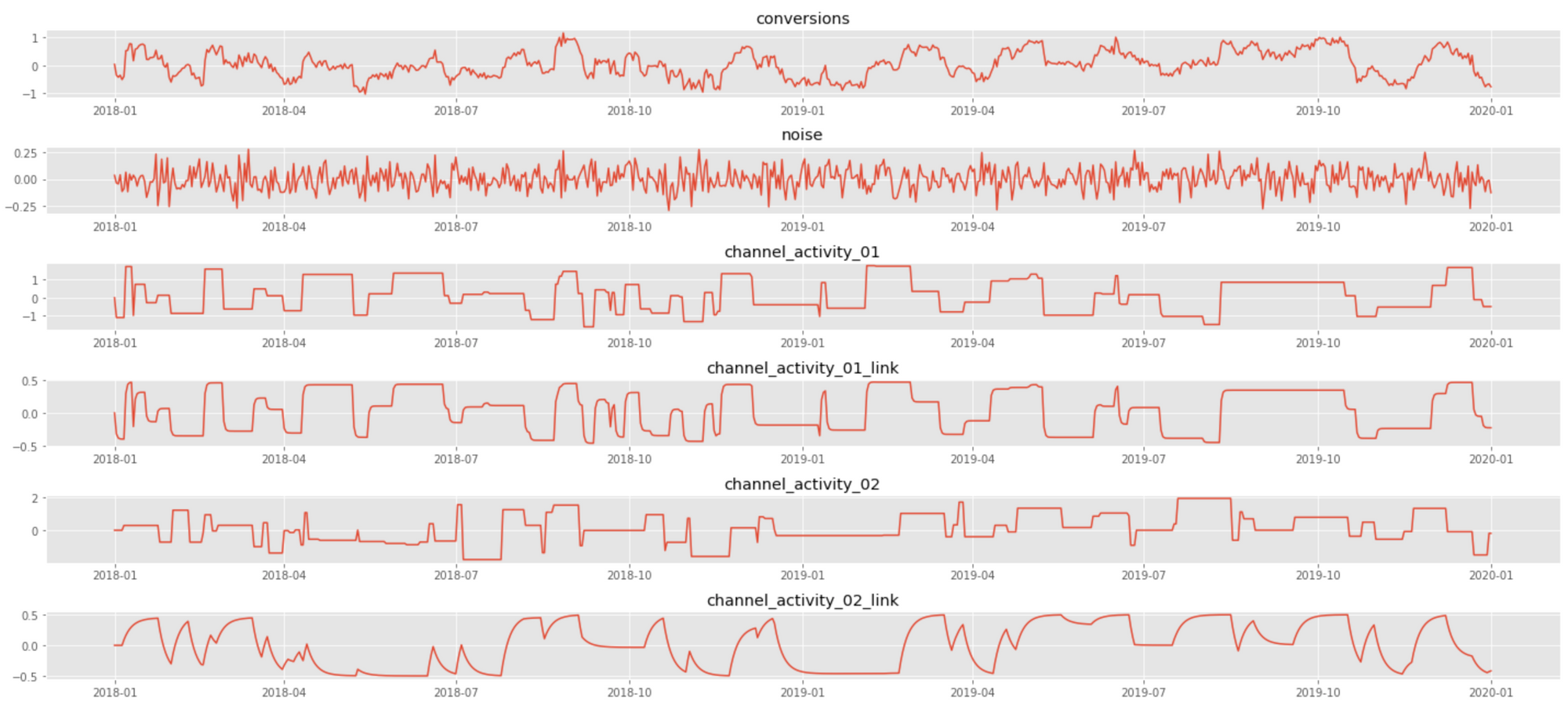
where $0<k_i<1$ and $\beta_i>0$ are the link function parameters for $i$th covariate, and $\alpha_0$ and $\alpha_i$ are the intercept and slope in the top-level regression, respectively. This model corresponds to a typical media mix model, where the signal is the number of conversions, covariates are marketing spends for different channels, sigmoid transformation accounts for saturation (diminishing returns), and convolution accounts for carryover (long-lasting) effects. The following plot shows a data sample that corresponds to the case of two channels with different saturation and carryover parameters:
We analyze the above signal using PyMC3, a probabilistic programming framework that greatly facilitates Bayesian inference by abstracting out many implementation complexities and providing a convenient modeling interface. The model specification in PyMC3 closely follows the mathematical notation we used above:
PyMC3 Model for Nonlinear and Memory Links. Click to expand the code sample.
import pymc3 as pm
import theano.tensor as tt

#
# sigmoid function (vectorized)
#
def saturation_link_tt(x, beta):
    return tt.nnet.sigmoid(tt.mul(beta.T, x)) - 0.5

#
# convolution operation (vectorized)
# we use the exponential kernel, but can be any function
#
def carryover_link_exp_tt(x, k, l = 30):
    w = tt.as_tensor_variable([ tt.power(k, i) for i in range(l) ])
    xx = tt.stack([ tt.concatenate([ tt.zeros(i), x[:x.shape[0]-i] ]) for i in range(l) ])
    y = tt.dot(w/tt.sum(w), xx)
    return y

#
# Data
#
x = df[['channel_activity_01', 'channel_activity_02']].values.T
y = df[['conversions']].values.T

#
# Model specification
#
with Model() as model:
    # parameters and priors
    beta = Gamma('beta', mu=10, sigma=5, shape=(1, num_channels))
    k = Beta('k', mu=0.5, sigma=0.2, shape=num_channels)
    alpha0 = Normal('alpha0', 0, sigma=20, shape=1)
    alpha = Gamma('alpha', mu=1, sigma=0.2, shape=(1, num_channels))

    # apply link functions
    x_saturated = saturation_link_tt(x, beta)
    x_linked = tt.stack( [ carryover_link_exp_tt(x_saturated[i,:], k = k[i])
                           for i in range(num_channels) ] )

    # top level regression
    likelihood = Normal('y', mu = alpha0 + tt.dot(alpha, x_linked), sigma=1, observed=y)
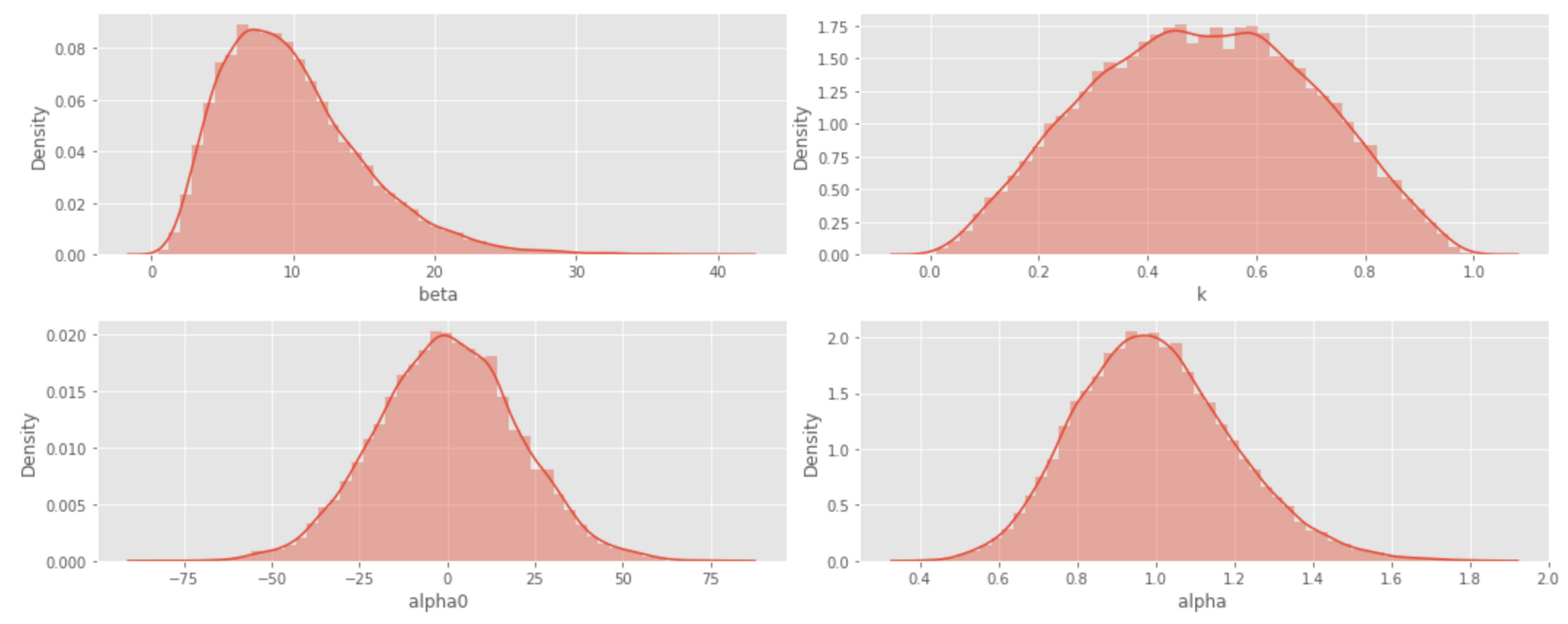
In the above model, we set relatively weak priors for all parameters. The corresponding probability densities are visualized in the histograms below.
Next, we fit the model using Markov Chain Monte Carlo (MCMC), as shown in the code snippet below.
PyMC3 Model Inference. Click to expand the code sample.
with model:
    trace = sample(3000, cores=4, init='advi')

with model:
    traceplot(trace)
The estimates produced in this way quite accurately reproduce the true parameters of the generator, which are $\beta_1=1.0, \beta_2=10.0, k_1=0.2, k_2=0.8$.
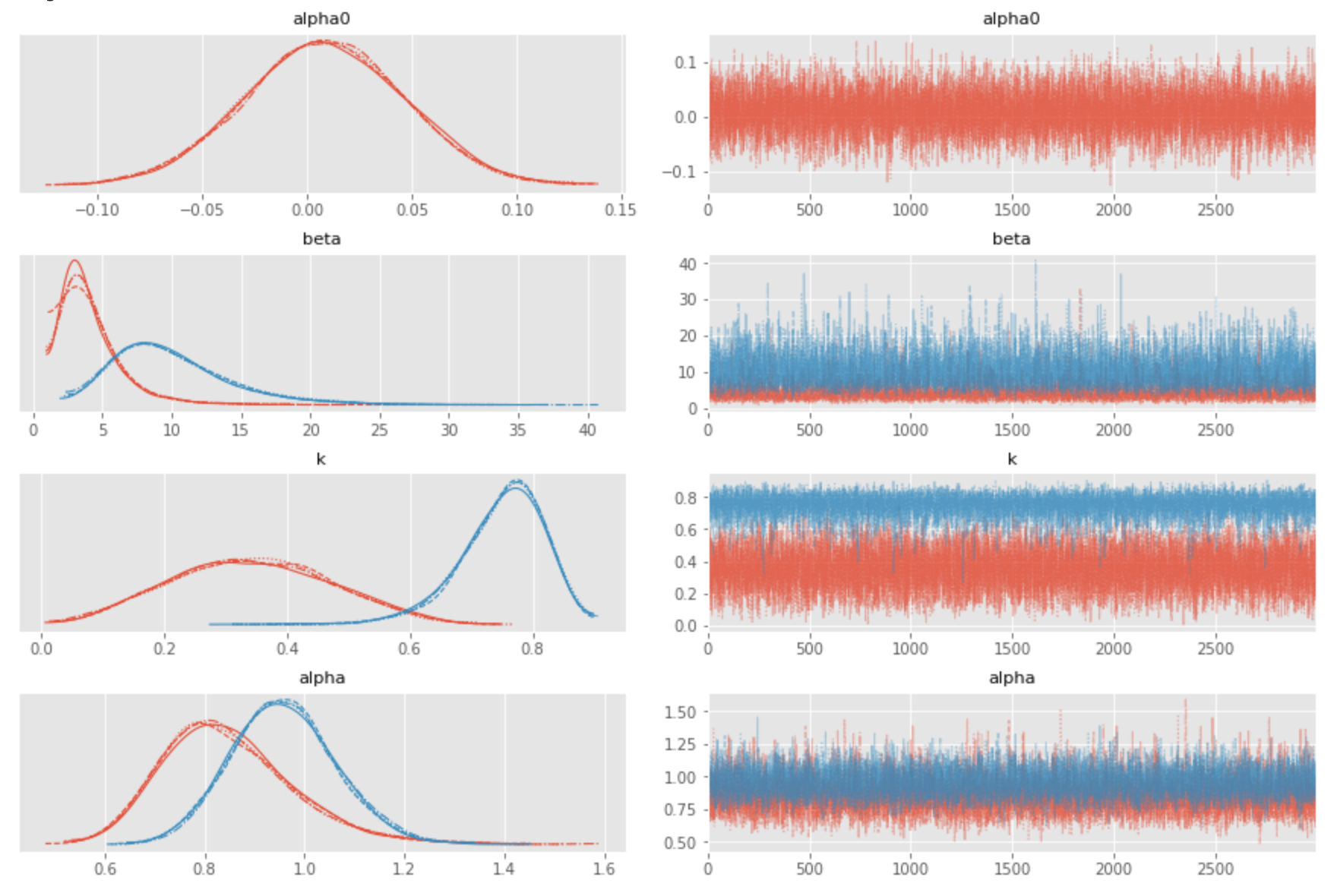
This example demonstrates the expressiveness of Bayesian inference: we can estimate saturation and carryover effects, separately or combined, using just a few lines of code. This basic solution can be extended in many ways to analyze more nuanced properties of the link functions, analyze autocorrelations in both signal and covariates, create forecasts, estimate forecast distributions, and more.
Analysis Using BSTS
The Bayesian model developed in the previous section is essentially a regression model that considers input samples to be independent. However, the input is a time series, and we generally need to account for the dependencies between the samples.
We partly incorporated this consideration into the model using the concept of a memory link; therefore, each sample of the signal was dependent on several adjacent samples of the covariates, which can be graphically summarized as follows.
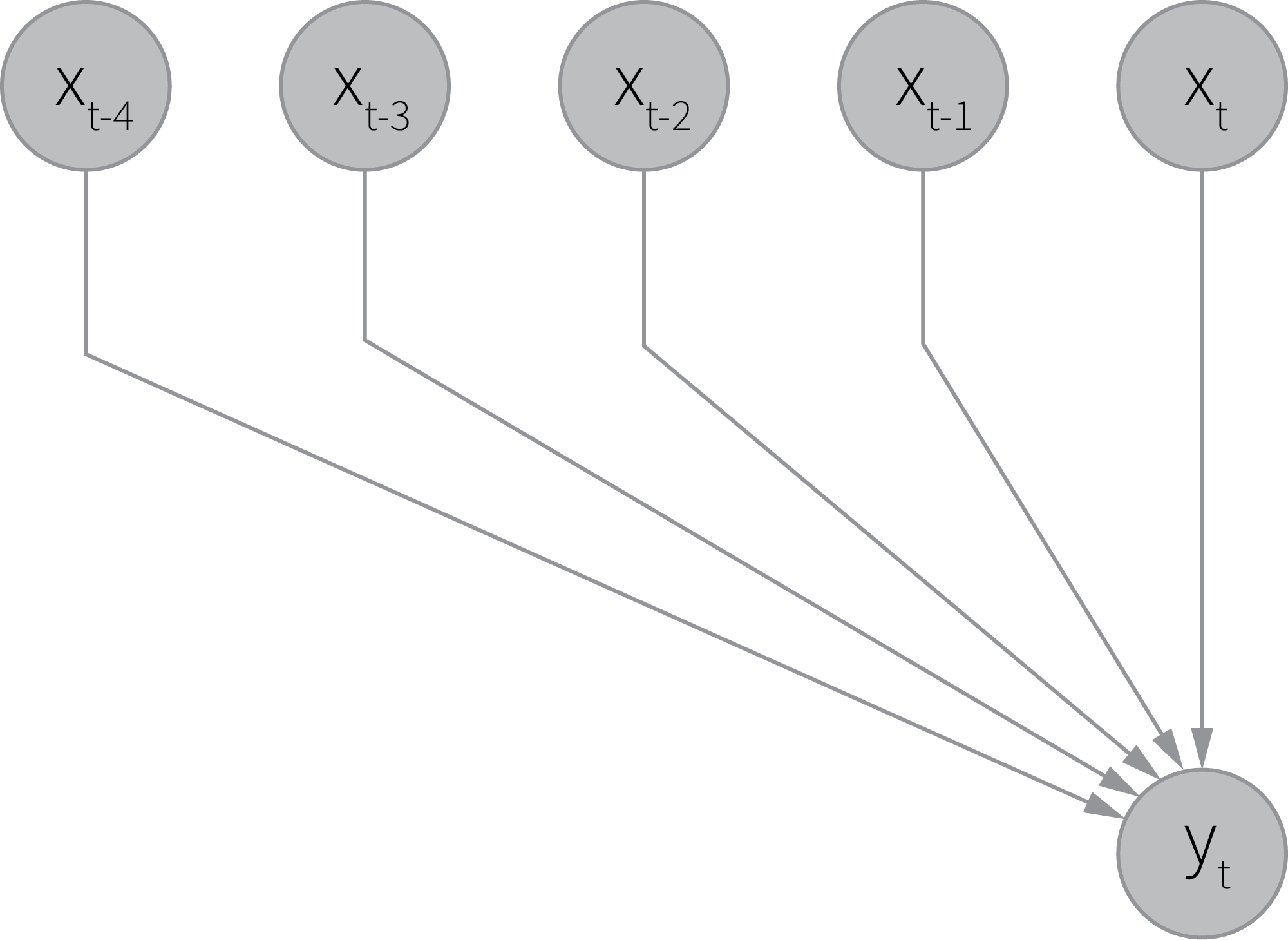
This approach works for simple cases where the observed signal is mainly a deterministic function of covariates, but it falls short when the signal is produced by a process with complex hidden dynamics that is only partly explained by the observed covariates. We can work around this problem by introducing a model wherein the process has a hidden state that stochastically evolves over time, and the observed signal is obtained as a projection of this state. The simplest model that implements this idea can be defined as follows:
$$
\begin{aligned}
s_t &= \phi s_{t-1} + \alpha x_t + w_t \\
y_t &= x_t + v_t
\end{aligned}
$$
where $x_t$ and $y_t$ are the observed covariate and signal, respectively, and $s_t$ is the unobserved state.
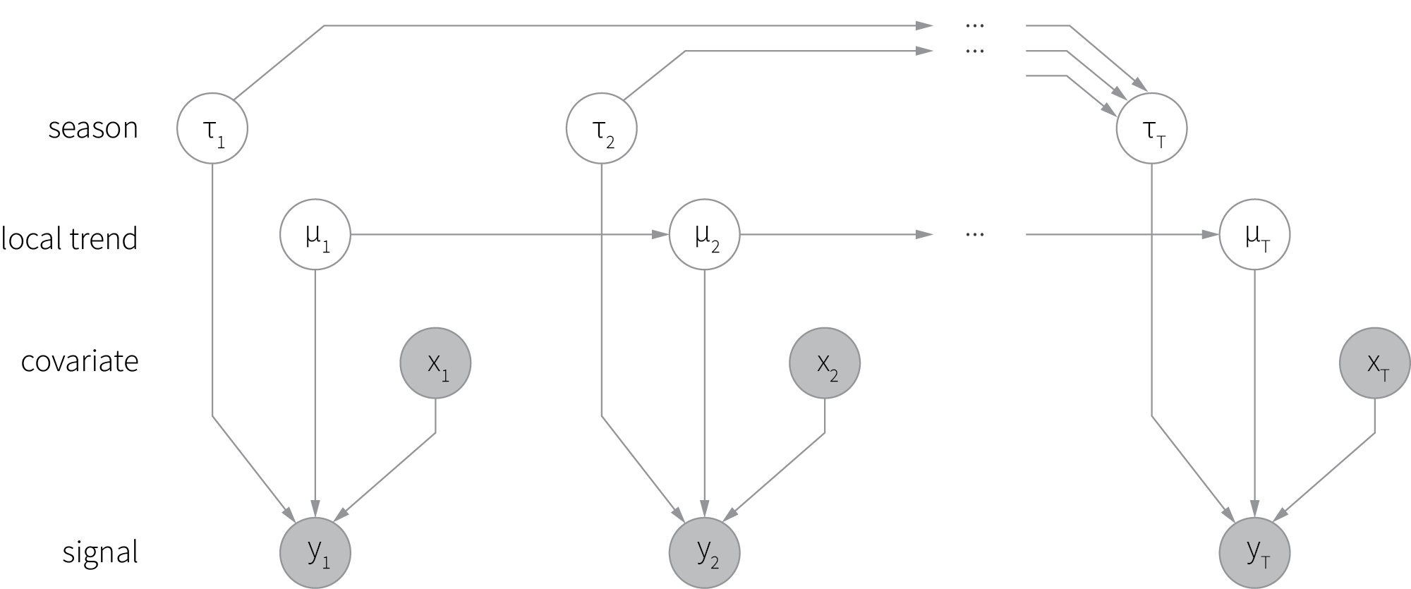
We can further entertain this idea and create a more complex model that includes multiple hidden processes, each of which has its own evolving state. This family of models is known as Bayesian structural time series (BSTS) and typically includes processes (components) such as trend, seasonality, and regression [7]. A graphical representation of a typical BSTS model is shown below (shaded circles correspond to the observed variables, and empty circles denote hidden variables).
Although the mathematical foundations of BSTS are quite complicated, probabilistic programming frameworks abstract out most of the implementation complexity. This is illustrated by a code snippet below, where we specify a BSTS model with trend, seasonality, and regression components using TensorFlow probability.
BSTS Model. Click to expand the code sample.
def build_sts_model(observed_signal, covariates):

    seasonal_effect = sts.Seasonal(
        num_seasons=52,          # weeks
        num_steps_per_season=7,  # days per week
        allow_drift=True,
        observed_time_series=observed_signal,
        name='seasonal_effect')

    trend_effect = sts.SemiLocalLinearTrend(
        observed_time_series=observed_signal,
        constrain_ar_coef_positive=True,
        name='trend_effect')

    covariate_effect = sts.SparseLinearRegression(
                    design_matrix=covariates,
                    name=f'covariate_effect')

    model = sts.Sum([seasonal_effect,
                     trend_effect,
                     covariate_effect,
                    ],
                    observed_time_series=observed_signal)
    return model
The above model can be extended with lagged regression components to analyze memory effects—please see the complete notebook for details.
A decomposition of a signal with seasonality, linear trend, two covariates with a linear link, and one covariate with a carryover link is shown in the figure below. The red line corresponds to the mean estimate of the component, and the blue band corresponds to its standard deviation. The covariate_effect component corresponds to the total contribution of all covariates (modeled as a linear regression).
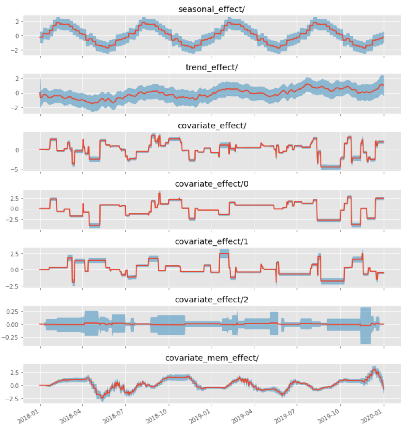
We can see that the BSTS model successfully decomposes the observed signal into hidden components and estimates the link functions. The same model can be used to build the forecast and estimate its uncertainty ranges. This versatility makes BSTS one of the best tools for enterprise time series analysis and decomposition.
Conclusions
We have discussed ten techniques for time series decomposition and interpretable forecasting. These techniques help to detect and analyze several effects such as saturation and carryover that are commonly present in enterprise data. We conclude this article with a brief discussion of how to choose the right set of methods for solving practical problems.
One consideration is the role of interpretability in a concrete solution. In some cases, we might be looking to enhance a black-box forecasting model; in others, the entire solution can be designed and implemented with explainability being the main and even the only goal. The best set of methods to be used is different in these two cases.
Another major consideration is the use case we build the model for. For instance, demand modeling often requires us to incorporate a large number of signals and account for seasonality, media mix modeling often requires us to incorporate prior assumptions, and customer analytics often benefits from even-level analysis. This influences both the model design and interpretation objectives.
Finally, one should take into account implementation complexity, computational stability, and data quality. Some methods such as GBDT are generally very robust; other methods such as Bayesian models might require careful tuning.
References
- Roger Koenker and Gilbert Bassett, “Regression Quantiles”, Econometrica, 1978
- Tony Duan, Anand Avati, Daisy Ding, Khanh Thai, Sanjay Basu, Andrew Ng, and Alejandro Schuler, “NGBoost: Natural Gradient Boosting for Probabilistic Prediction”, 2020
- Lloyd Shapley, “A value of n-person games. Contributions to the Theory of Games”, 1953
- Scott Lundberg and Su-In Lee, “A Unified Approach to Interpreting Model Predictions”, 2017
- Jerome Friedman, “Greedy function approximation: A gradient boosting machine”, 2001
- Tobias Lang and Matthias Rettenmeier, “Understanding Consumer Behavior with Recurrent Neural Networks”, 2017
- Kay Brodersen, Fabian Gallusser, Jim Koehler, Nicolas Remy, and Steven L. Scott. "Inferring causal impact using Bayesian structural time-series models", 2015
