Multi-agent deep reinforcement learning for multi-echelon supply chain optimization

Supply chain optimization is one the toughest challenges among all enterprise applications of data science and ML. This challenge is rooted in the complexity of supply chain networks that generally require to optimize decisions for multiple layers (echelons) of distribution centers and suppliers, multiple products, multiple periods of time, multiple resource constraints, multiple objectives and costs, multiple transportation options, and multiple uncertainties related to product demand and prices. In the traditional approach, one usually develops a mathematical programming model that explicitly incorporates a relevant subset of these factors and obtains a solution through solving this model using optimization and forecasting methods. An extensive survey of such models is provided, for instance, in [1].

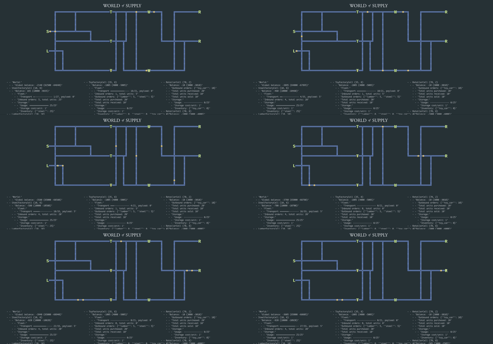
In this article, we explore how the problem can be approached from the reinforcement learning (RL) perspective that generally allows for replacing a handcrafted optimization model with a generic learning algorithm paired with a stochastic supply network simulator. We start by building a simple simulation environment that includes suppliers, factories, warehouses, and retailers, as depicted in the animation below; we then develop a deep RL model that learns how to optimize inventory and pricing decisions.

This work builds on the basic example we developed in one of the previous posts, and the complete implementation is available on GitHub as part of the TensorHouse project.

Simulation Environment

Our first step is to develop an environment that can be used to train supply chain management policies using deep RL. We choose to create a relatively small-scale model with just a few products and facilities but implement a relatively rich set of features including transportation, pricing, and competition. This environment can be viewed as a foundational framework that can be extended and/or adapted in many ways to study various problem formulations. Henceforth, we refer to this environment as the World of Supply (WoS).

The design of the WoS environment is outlined in the following class diagram and described in detail below:

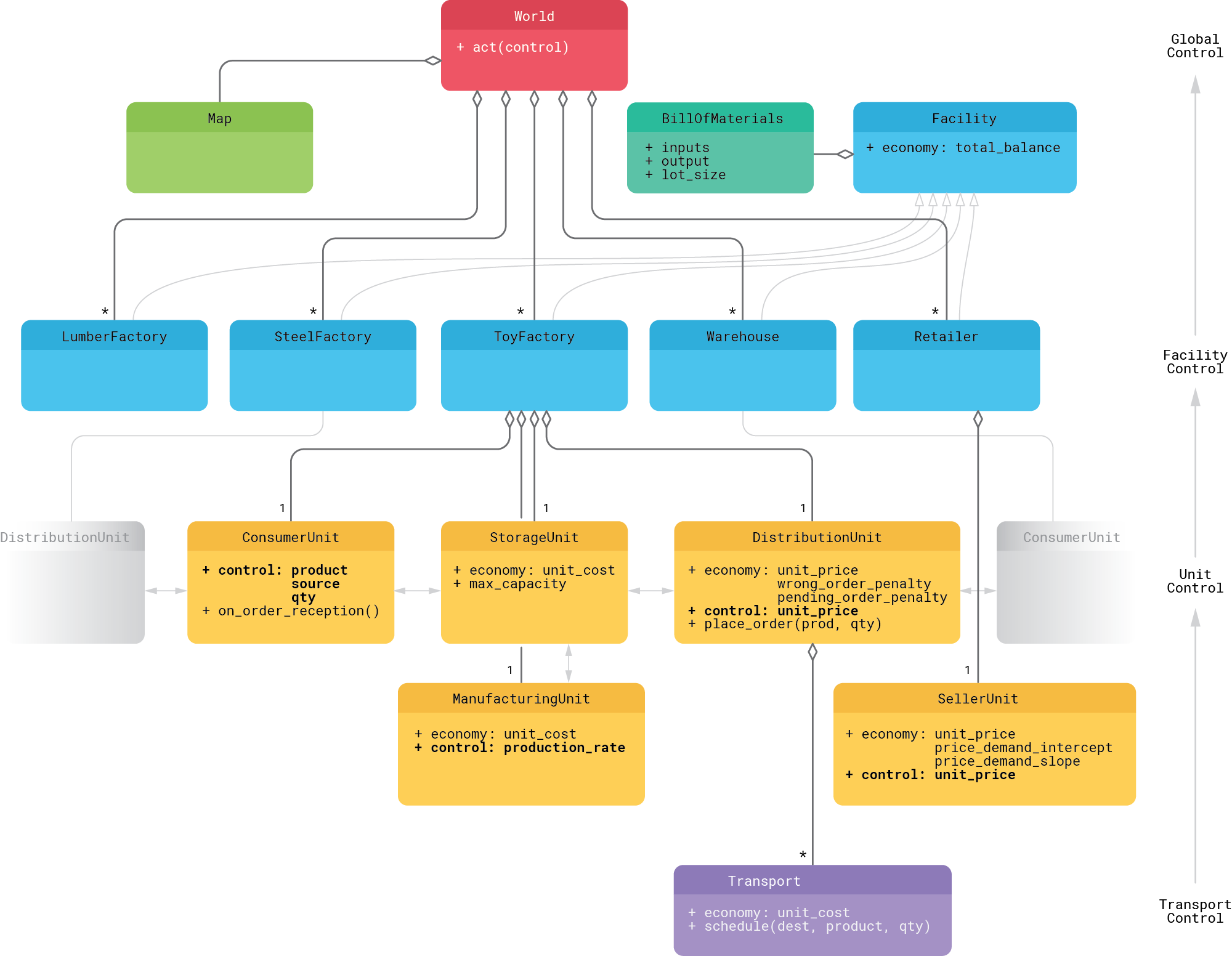
• The root entity of the environment is the World that consists of a Map and Facilities. The Map is a rectangular grid layout that specifies locations of the facilities and a transportation network (railroads) that interconnects these facilities. The grid-based layout is chosen mainly for the convenience of visualization, and it can be straightforwardly replaced by a more realistic graph-based connectivity map for larger-scale experiments.
• Each Facility is essentially a collection of Units that model the different aspects of operations: procurement (consumption) from upstream suppliers, storage, manufacturing, distribution to downstream consumers, and selling to the end customers. The composition of units is different for different facility types. For instance, producers of raw materials do not have Consumer units and Retailers do not have Manufacturing units.
• Each Facility has a Bill of Materials (BOM) that describes its inputs and outputs. For example, a BOM can state that a factory consumes one unit of lumber and one unit of steel to produce one unit of toy cars. Each Facility also has an Economy that encapsulates cost and price related parameters and logic, in particular its total balance.
• Storage unit keeps track of the inventory available at the Facility and keeps track of storage costs.
• Manufacturing unit takes inventory from the storage, assembles the output according to the BOM, and places this output back to the storage. The unit tracks manufacturing costs, and the control policy can change its production rate (number of lots assembled at each time step).
• Consumer unit places orders to upstream suppliers (sources), one at a time. It requires the control policy to specify product ID, source ID, and product quantity.
• Distribution unit receives and fulfills the orders placed by upstream consumer units. It charges consumers a certain price per unit, which is managed by the control policy, charges a penalty for wrong orders (in case the facility does not produce the ordered product), and charges its own facility for all open (unfulfilled) orders at each time step. The distribution unit also owns a fleet of Transports that delivers the products to consumers.
• Finally, the Seller unit exposes the inventory to the outside world. Its Economy module encapsulates the price-demand function and the control policy needs to manage the selling price.
• For the optimization process described in the next sections, we use a small-scale instance of a network that includes a lumber mill, steel mill, toy factories that assemble toy cars from lumber and steel, warehouses (distribution centers), and retailers. This setup has nine facilities in total.

Almost all entities in the above environment, including the World, Facilities, Units, and Transports are agents in terms of RL, and so this is a hierarchical multi-agent environment. For the training process described later in this article, we simplified the control space by automating Transports (vehicles automatically find the shortest path for each order and deliver the freight); however, logistics decisions can be directly included into the optimization process.

Although the environment described above is fairly simple, the optimization of control policy is complicated by the dependencies between agents and progress-blocking traps. For instance, global profit optimization requires all layers of the network to operate in concert, so that the downstream facilities (e.g., retailers) will not be able to earn anything and learn their policies until the suppliers (e.g., warehouses) learn their policies, which in turn cannot be accomplished until the whole chain works and downstream facilities sell products to the end customers. Other examples of progress-blocking traps include storage overfills that block inbound inventory flows and can also block vehicles at the unloading state.

States, Models, and Policy Mappings

Our second step is to create an adapter that casts the WoS environment to the standard environment interface provided by RLlib—a reinforcement learning platform that we will use for policy training. This interface is similar to OpenAI Gym but provides comprehensive multi-agent features.

One of the design decisions we need to make is the mapping between agents and policies. The nested structure of the WoS environment allows for a variety of mapping schema. One extreme is to map the entire World to a single policy that would need to produce a high-dimensional action vector that comprises all controls for all facilities. Another extreme is to map each Unit or each Facility to its own policy. After experimenting with various mappings, we concluded that it makes sense to maintain a balance between the dimensionality of the action space and the number of independent policies. One schema that achieves reasonably good performance is shown in the illustration below:

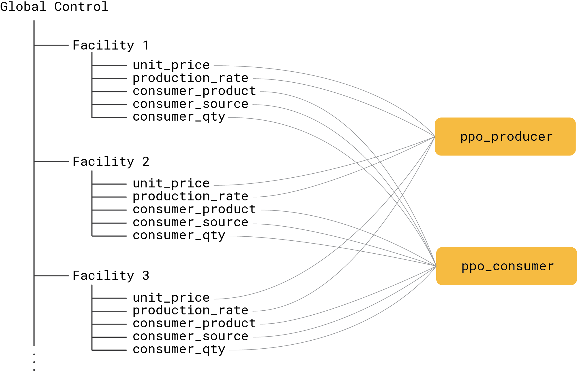
This schema maps all production-related controls to one policy, and all consumption-related controls to another policy. This reduces the dimensionality of the action spaces; thus, we have one 2-dimensional and one 3-dimensional action space. The policies of course need to take the type and location of each facility into account, but we handle this in the design of the state.

Next, we use the proximal policy optimization (PPO) algorithm for both producer and consumer policies [2]. The design of the state representation and network architecture for the consumer policy is shown in the figure below:

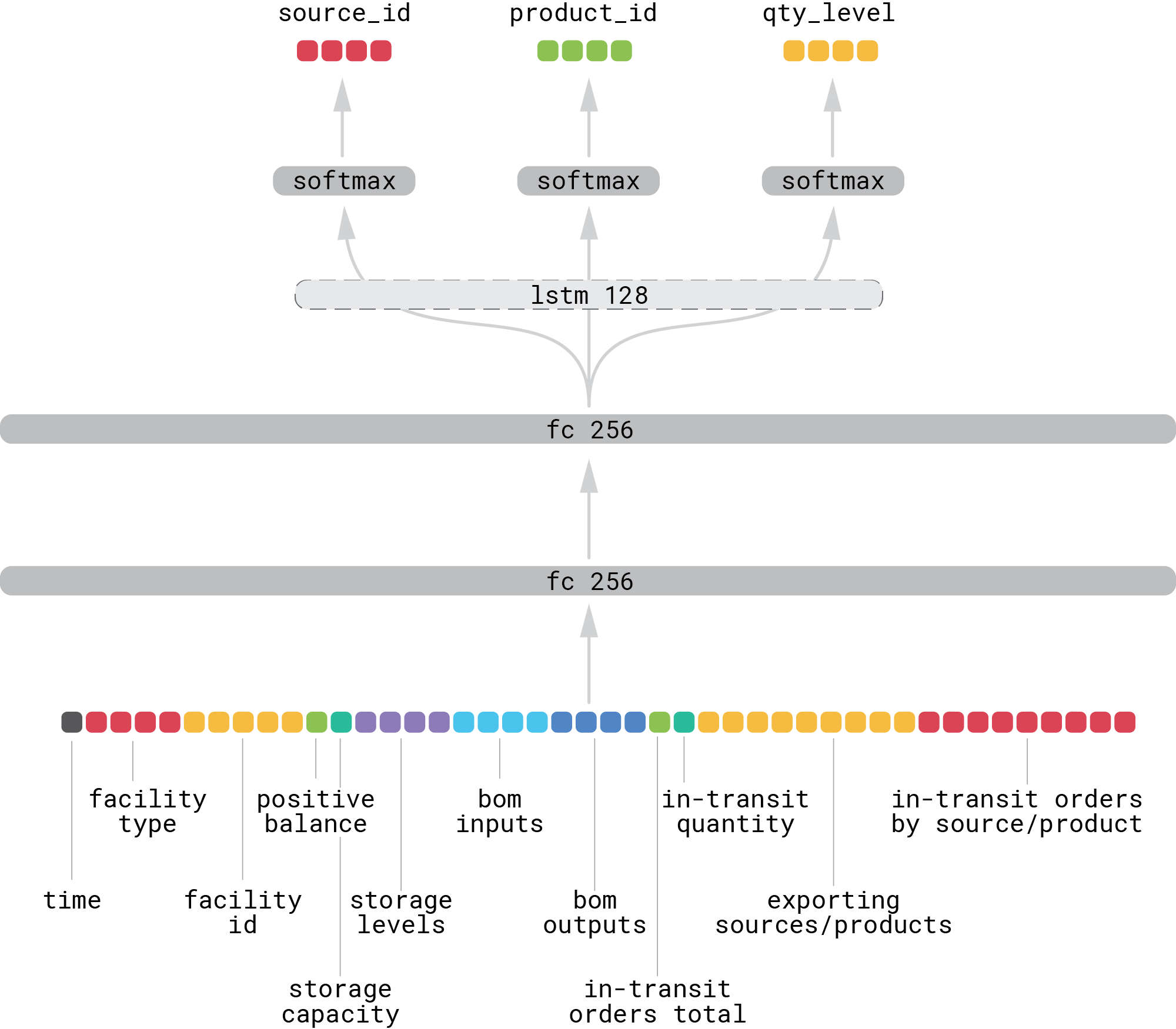
The state vector includes global features such as time; a comprehensive set of facility-level features, such as one-hot encoded facility type and identity; BOM inputs and outputs; information about which sources export which products; and what orders are already in transit. The model consists of two wide fully connected layers, and their outputs are mapped to three short linear layers with softmax on top to produce the probabilities of source ID, product ID, and quantity level—the consumer unit then assembles an order from these three values. In general, one can benefit from an LSTM layer that captures the temporal dynamics of the environment—similar to OpenAI Five [3]—however, we did not observe any significant improvement for the setup we used in the experiments described in the next sections. The producer network has a similar design but smaller dimensionality of the fully connected layers.

We use multi-discrete action spaces for both policies, so that product quantities and prices are drawn from a discrete set, although one can consider using continuous control spaces for these elements.

Finally, we use simulation episodes with 1,000 time steps that are downsampled by a factor of 20 before being fed into the policy, so that the policy makes 50 decisions per episode.

Baseline Policy

Our third step is to implement a hand-coded policy that can be used as a baseline and, as we will see later, a bootstrapping mechanism for learning PPO policies. The hand-coded policies implement a very simple logic:

• The producer policy has fixed production rates and unit prices for each facility type that are manually chosen in a way that results in reasonably good performance.
• The consumer policy calculates ratios between the number of product units available in storage and the number of units required according to the BOM and orders the most-needed input product from a source randomly chosen among all facilities that export this product.

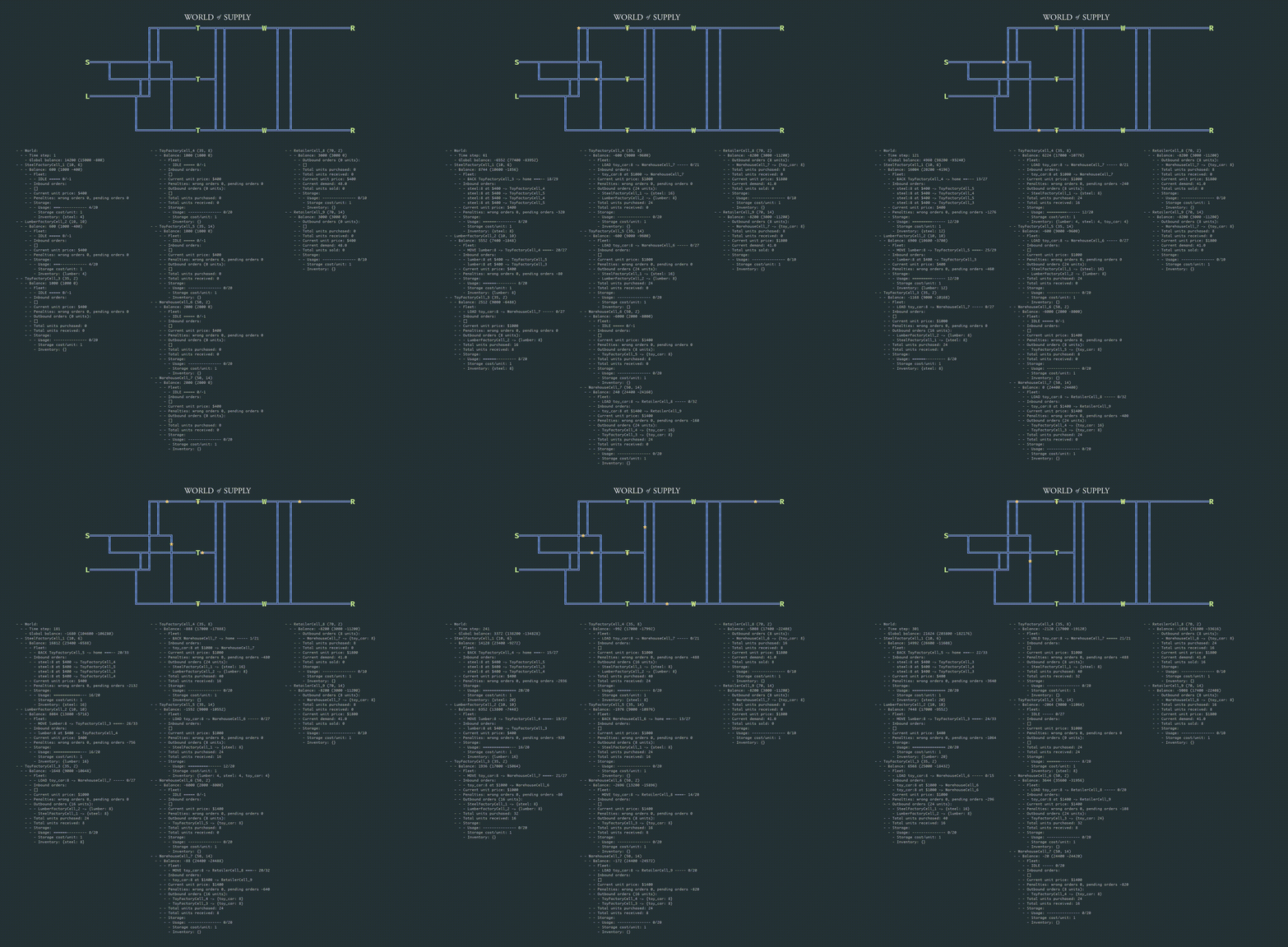
The following animation shows the debugging information for the begging of one episode (300 steps out of 1,000) played by a hand-coded policy:

Rewards and Training Process

The deadlocking dependencies between facilities make the training process challenging, but we can leverage several techniques to work around it.

First, we need to design the reward signal. The WoS environment provides flexibility to determine how exactly the optimization goal can be set: we can view the entire network as a retailer's supply chain and ignore the profitability of individual facilities, or we can view it more as an economic game where each facility is an independent agent that aims to maximize its own profit. We choose to focus on global profit, that is, the sum of all revenues and losses across all facilities. Direct maximization of global profit, however, can be challenging because of significant delay between a facility’s actions and profits ultimately obtained at the end of the chain. As a result, agents tend to get stuck at local do-nothing minimums to minimize losses. We can facilitate the process using curriculum learning—start with easier subtasks and gradually increase the difficulty level. The following example shows a reward signal design based on these considerations:

$$
\begin{aligned}
\alpha &= \alpha_0 + \alpha_1 \cdot \frac{t}{T} \\
r_g &= \alpha\cdot p_g + (1 - \alpha) \cdot p_r \\
r_i &= \beta \cdot r_g + (1 - \beta) \cdot p_i
\end{aligned}
$$

where $\alpha$ is the weight of global profit that increases during the training process ($\alpha_0$ and $\alpha_1$ are the intercept and slope of the linear growth function, $t$ is the training iteration, $T$ is the total number of training iterations), $p_g$ is the global profit, $p_r$ is the mean retailer’s profit or revenue, $p_i$ is the own profit of $i$-th facility, and $r_i$ is the final reward metric for $i$-th facility. In words, we initially focus on ensuring that the supply chain is functioning end to end and retailers make a revenue of $p_r$ and then shift the focus toward the global balance. The local balance of a facility is essentially a regularizer controlled by a constant parameter $\beta$.

The reward design is illustrated in the plots below that show how the global balance, total reward, and rewards of individual agents evolve during the first half of the episode (500 steps) under the baseline policy:

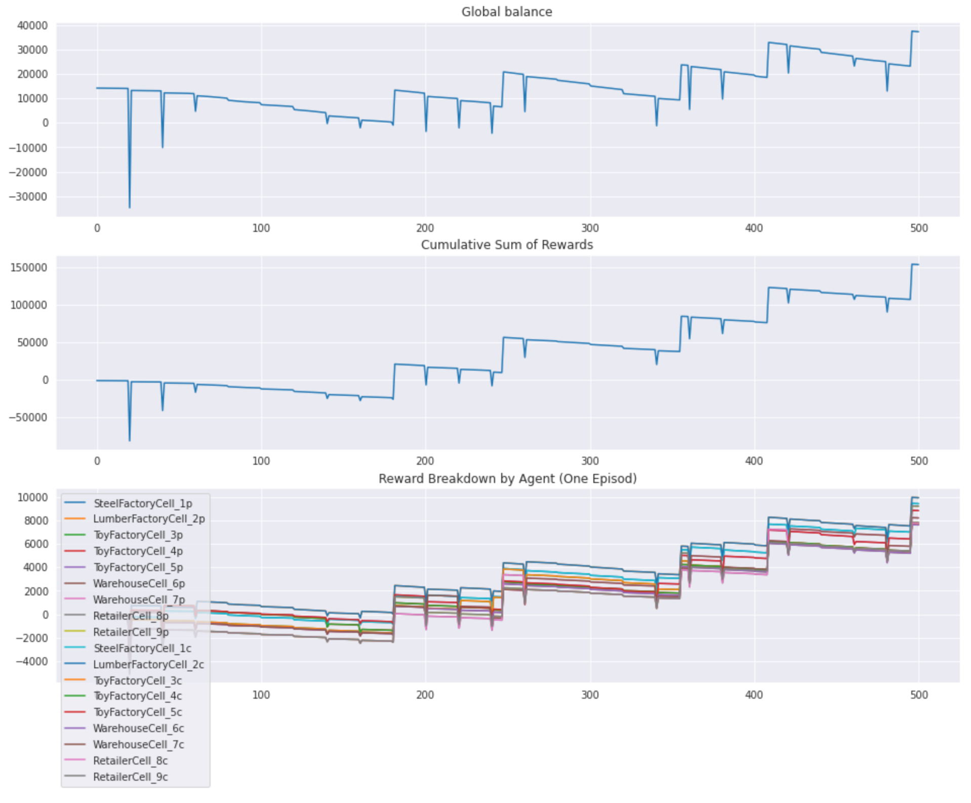
Note that each facility is represented by two agents (in RL terms) because we have separated producer and consumer policies, and, in general, one can have different definitions of reward for producer and consumer actions.

The second technique we use is also based on a curriculum learning approach: we initially assign the baseline policy to all agents to ensure the basic functioning of the network, and gradually switch groups of facilities from the baseline to the PPO policies (e.g., toy factories first, distribution centers second, etc.).

Results and Discussion

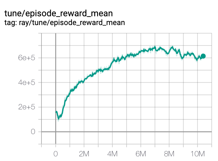
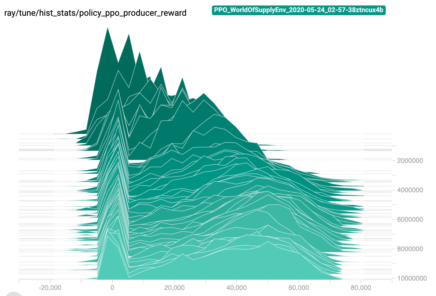
The training process is generally able to produce a meaningful policy for one layer of facilities (e.g., toy factories) in about 300,000 episodes. The reward trajectory has an inverted-U shape as we start with the revenue-focused rewards and gradually increase the contribution of profits. This process is illustrated in the two figures below that show the dynamics of the mean and distribution of the episode reward for one training session:

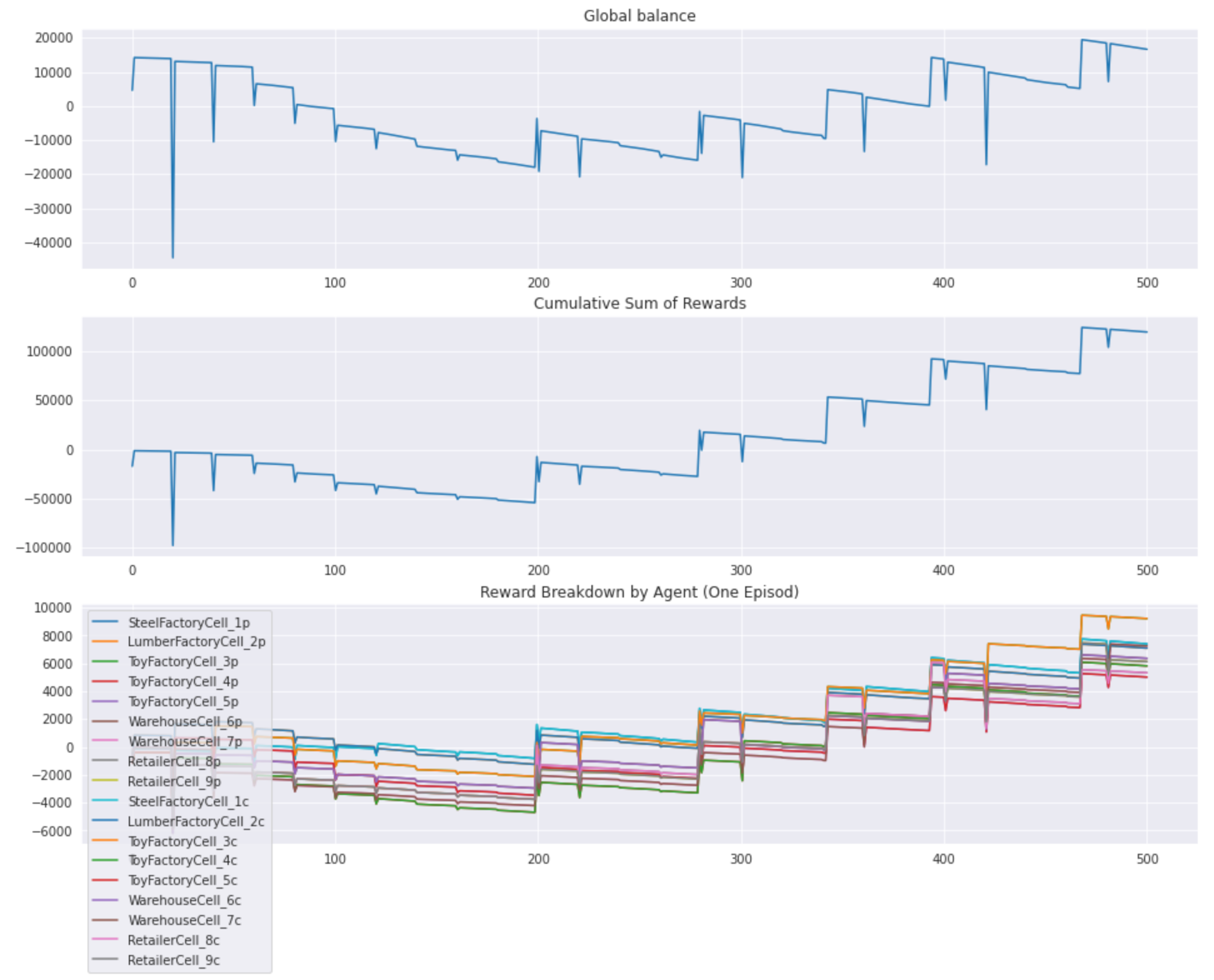
The learned policy demonstrates reasonably good performance, but we did not manage to outperform the baseline policy. The overall supply chain profit performance under the learned policy is inferior to the baseline because of imperfect selection of suppliers that results in order placement penalties and occasional progress collapses caused by environment blocking. The plots below show an example of balance and reward traces that can be contrasted to the baseline policy traces provided in the previous section:

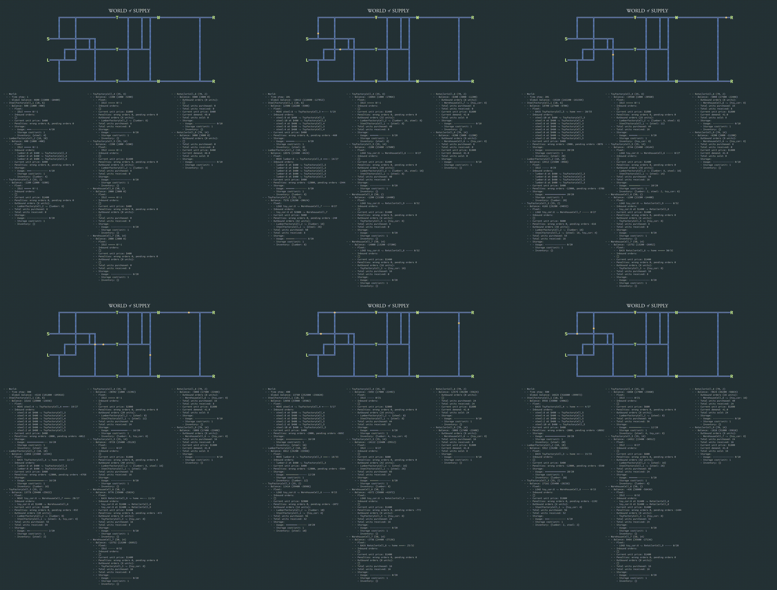
The animation below provides a detailed view with the debugging information:

Once the policy for one layer of facilities (echelon) is stabilized, the process can be repeated for another layer or group of facilities, and so on.

The experiments above show that it is generally possible to apply multi-agent RL methods to multi-echelon supply chain optimization, but there are a number of challenges that need to be addressed:

• Action spaces and agent coordination. Any realistic supply chain represents a complex environment that can be mapped to decision-making agents in various ways. This mapping is associated with a trade-off between the complexity of individual agents and coordination between the agents. A small number of agents generally lead to high-dimensional action spaces that are challenging to handle using most of the standard RL algorithms. On the other hand, a large number of agents result in a coordination challenge where the agents are chained together and cannot make progress independently of each other—a normal scenario in real-life supply chain applications.
• Progress blockers and reward design. Realistic supply chain environments can have irreversible progress blockers or other nonsmooth state-action-reward dependencies. For instance, inventory overflows can block the transportation process. This makes the multi-agent training problem even more challenging because the blockers tend to trigger a domino effect. This issue relates to the reward design as well, because local (selfish) rewards tend to drive agents into globally nonoptimal or blocking behavior. As we discussed in the previous sections, the problem can be mitigated by using curriculum learning techniques that ensure global progress before improving performance.
• Low-level vs high-level controls. The challenges described above can be more or less pronounced depending on how the environment is controlled. For instance, the design described above assumes that the policy directly manages many minor details: what item should be ordered, from what source, in what quantity, etc. An alternative is to wrap these low level controls into more intelligent or automated components and make the RL-generated policy manage the parameters of these components. For instance, the ordering process can be governed by an (s, Q) policy with reorder point and reorder quantity parameters dynamically or statically set by the RL-generated policy. This approach can sharply reduce both the dimensionality of the action space and the probability of performance collapses, as well as improve policy stability and interpretability (which are two other major challenges).
• Combinatorial optimization. Many of the above challenges stem from the combinatorial nature of the problem, i.e., the necessity to select actions from a discrete set with a large branching factor. This suggests that using the techniques and architectures geared toward combinatorial optimization, such as Monte Carlo Tree Search (MCTS) and other AlphaZero concepts, may be beneficial [4].

References

1. Josefa Mula, David Peidro, Manuel Díaz-Madroñero, Eduardo Vicens, “Mathematical Programming Models for Supply Chain Production and Transport Planning,” European Journal of Operational Research, 204(3):377–390, 2010.
2. John Schulman, Filip Wolski, Prafulla Dhariwal, Alec Radford, Oleg Klimov, “Proximal Policy Optimization Algorithms,” 2017.
3. https://openai.com/blog/openai-five/
4. David Silver, et al., “Mastering Chess and Shogi by Self-Play with a General Reinforcement Learning Algorithm,” 2017.