How to build and evaluate a Next Best Action model for customer churn prevention

Providing each customer with personalized treatment that helps improve long-term engagement is one of the most fundamental problems in marketing communications. This task is particularly important for businesses that rely heavily on long-term customer relationships, including telecom, video games, insurance, retail banking, and healthcare, as the costs associated with customer attrition are especially high. It is generally challenging to develop a model that automatically prescribes the next best action for each customer because we need to quantify the true impact of various actions, and it is particularly difficult to evaluate the efficiency of such models before they are actually deployed in production based on historical data. In this article, we describe the design of the next best action model that we commonly use in practice and elaborate on the methodology for offline efficiency evaluation.

Business Problem Overview

Next best action models are used for a wide range of marketing tasks, including content personalization, decision support tools for customer support specialists, and offer targeting. For the sake of specificity, we focus on the problem of customer churn prevention—we assume a business model in which customers regularly interact with the services provided by a company, and the goal is to identify customers with a high propensity to either decrease the intensity of service usage or explicitly cancel their accounts, and then determine the optimal personalized treatment for each of such cases.

We assume the availability of a customer database in which each customer profile includes the history of interactions (e.g., service usage, customer support calls), the history of treatments received by the customer (e.g., retention offers), and a binary label that indicates churn. The churn label can be computed based on the intensity of service usage (e.g., sharp decline over the last month) or on explicit account cancellation events. We further assume that past treatments were assigned using a black box system with test and control groups, but we do not know the exact logic for the test/control assignment or the treatment assignment. This situation is quite typical because the treatments can be managed by different departments, teams, and systems, both manually and automatically. The overall setup is summarized in the following figure:

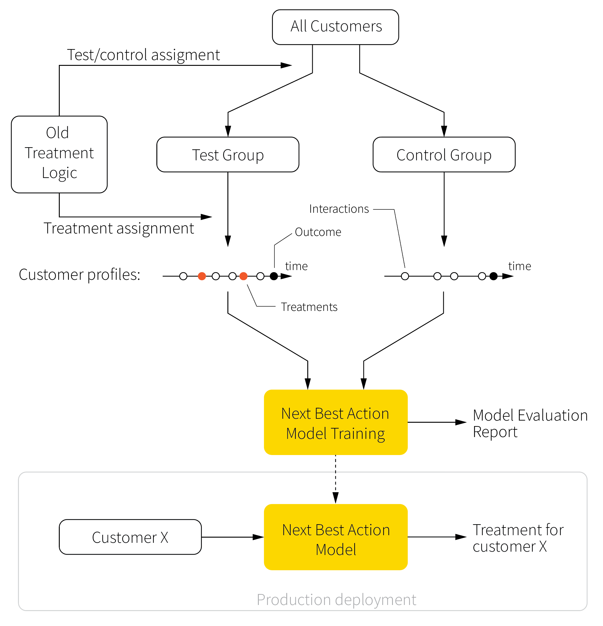
Our main goal is to develop the next best action model that prescribes the optimal treatment for a given customer based on their profile and to evaluate this model based on historical data. The main purpose of evaluation is to provide certain guarantees about the efficiency of the model before it is deployed in production.

Solution Architecture

The environment described in the previous section imposes several challenges. First, we do not know the logic used for the test/control assignments, and there is no guarantee that this assignment was random. Consequently, the historical data can have arbitrary biases. Second, we need to evaluate the performance of the model based solely on historical data. Ideally, we want to evaluate every model version in production using randomized experiments, but such testing is generally expensive and risky from a customer experience standpoint. Therefore, we have to develop a good offline evaluation methodology that reduces the number of online trials and mitigates the risk of deploying catastrophically wrong treatment policies.

We address the above challenges in four steps. First, we implement a procedure for bias control and correction that addresses potential biases in the historical data. Second, we build a core model that estimates the churn risk conditioned on different types of treatments, which further helps determine the optimal treatment strategy for each customer. Third, we implement the treatment selection logic based on the risk scores (the prescriptive part of the next best action model). Finally, we develop the evaluation procedure to assess the quality of the model based on the bias-corrected data. This architecture is outlined in the figure below.

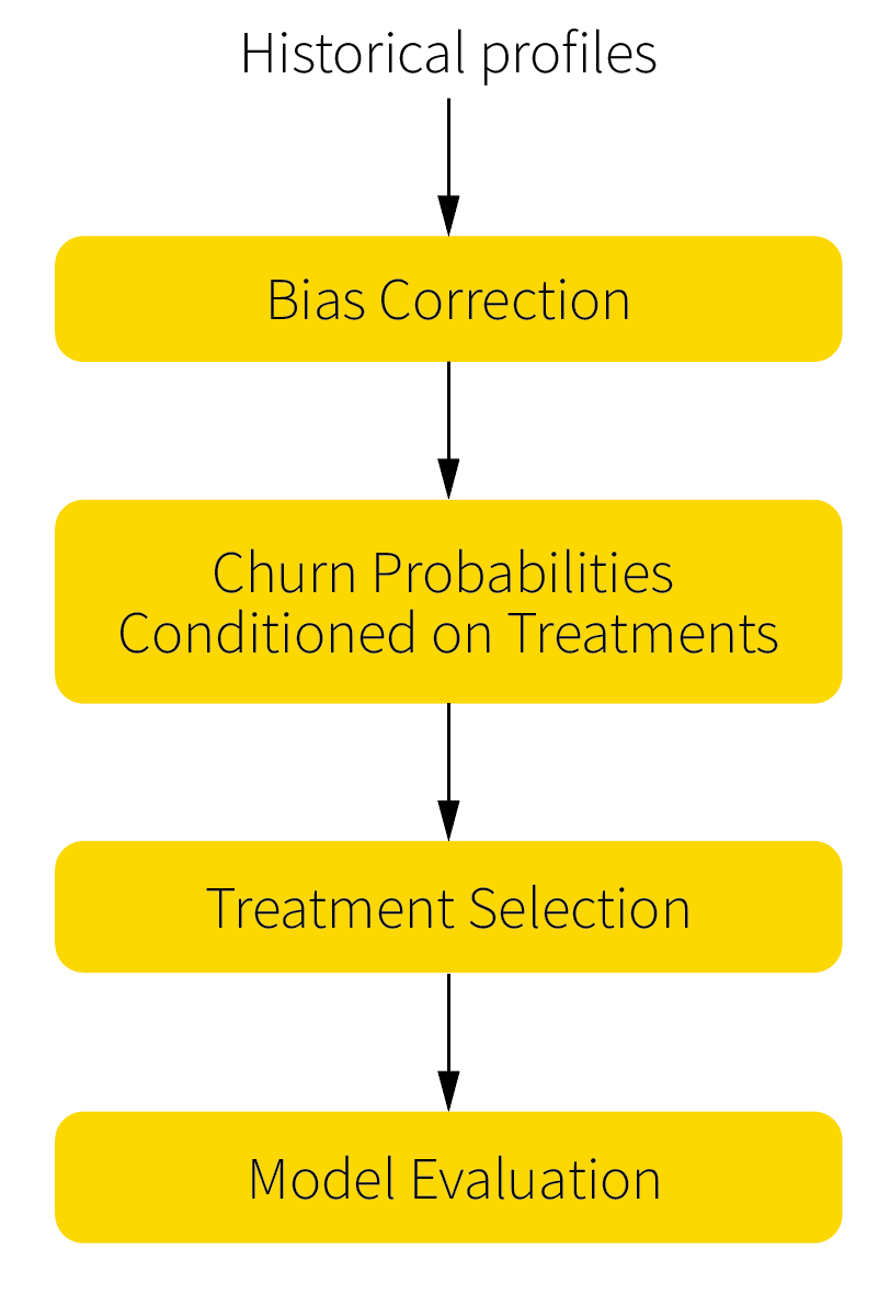
It should be noted that this solution optimizes one treatment at a time for any given customer and does not attempt to strategically optimize sequences of treatments. The elements of strategic optimization can be added on top of this solution using reinforcement learning techniques, but such an extension may or may not be practically feasible, depending on the available data volumes and other factors.

Bias Correction

Why do we need bias control and correction procedures, and why could we not use historical data directly? To evaluate the treatment effect, it is necessary to quantify how a specific treatment impacts the behavior (measured in terms of conversions, churn events, or other outcomes) of a specific customer. Conceptually, we should do the following experiment: do not treat a certain group of customers, observe the outcomes, go back in time, treat the same customers, and observe the alternative outcomes. Such an experiment is, of course, purely imaginary and cannot be performed in real life.

The alternative solution is to perform a controlled experiment. In a controlled experiment, there is only one variable that changes between the test and control groups, and all other variables are held constant. Usually, there is one control group and one or more test groups that are identical to the control one and different by only one variable. In our case, the only variable that should be changed is treatment (or different types of treatments), and the result should be compared with that of the group without treatment.

Near-perfect controlled experiments can be arranged, for instance, in physics, but dealing with customers’ demographics and behavior is challenging because it is generally not possible to find absolutely identical customers to ensure that the treatment is the only one factor that influences the churn level. In social studies and clinical trials, this issue is solved by random selection of participants for the test and control groups. This means that all participants should have an equal chance of taking part in each group. The perfect randomization ensures that there is no bias and that the effects of factors other than the main one (treatment in our case) are limited.

In marketing applications, a perfectly randomized experiment with a sufficient sample size for each kind of treatment and control group can be prohibitively expensive and time consuming. The alternative is to sample the test and control groups from historical data and make a comparison. The sampling can be done through the selection of treated and non-treated customers from historical data to form test and control groups, respectively. In this case, we need to ensure that the data are not biased, or if they are biased, we need to make a correction to reduce the difference between the groups.

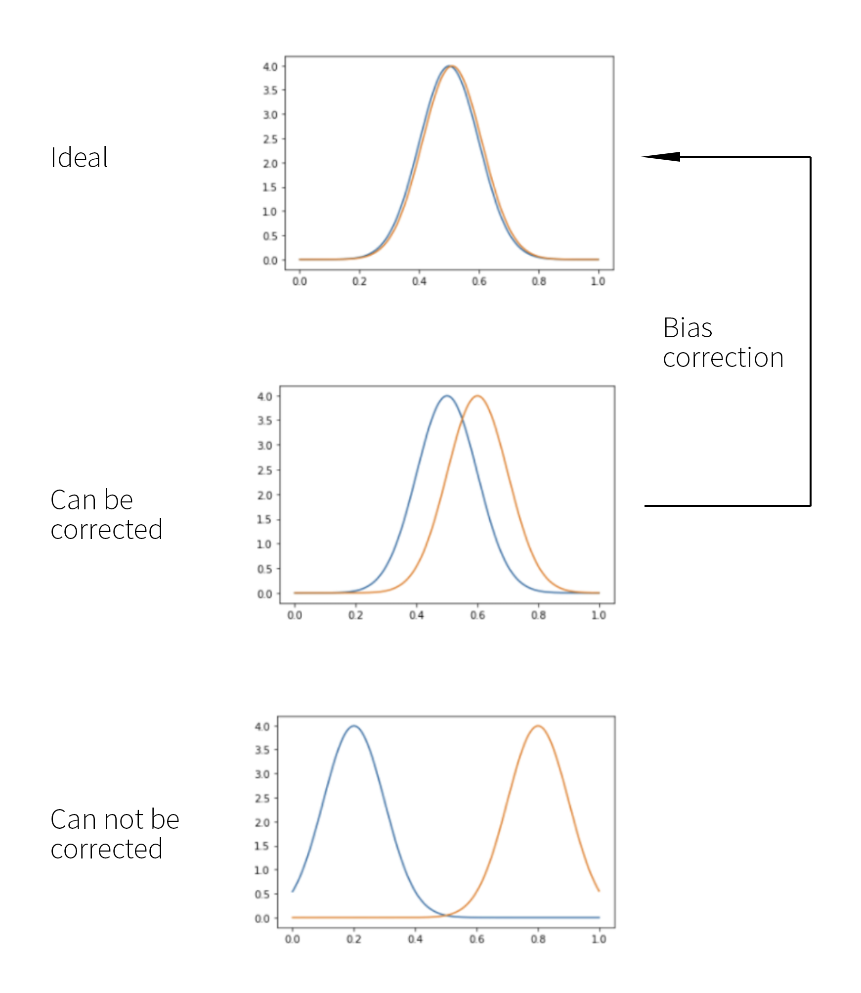
We can start by drawing a random sample of the test and control groups and by fitting an arbitrary classification model to predict test and control (that is, treatment and non-treatment) labels. For example, we can use gradient-boosted decision trees to build such a model. The accuracy of the model, that is, its ability to predict the test/control label based on customer profile features, can then be viewed as a measure of bias, and the following three cases are possible:

1. The accuracy is very low, so the probabilities of the test and control classes predicted by the model are roughly equal across the population. This suggests that the test and control groups can be viewed as unbiased, and we can proceed with regular churn modeling.
2. The model can differentiate between the test and control groups to a limited extent so that the probabilities of two classes diverge. This indicates the presence of a limited bias that can be corrected.
3. The model can predict test/control label relatively well, and the class probabilities diverge considerably. This indicates that the data are heavily biased, and it might not be possible to correct such a bias.

The above categorization is summarized in the following figure:

Let us assume that we have sampled the test and control groups from historical data, assessed the bias, and observed that the magnitude of the bias is high enough to require correction but not high enough to make such a correction impossible. There are three main ways to make a correction:

• Reverse engineering of groups’ selection process
• Heckman correction
• Propensity score matching

Reverse engineering of groups’ selection process

It is sometimes possible to reproduce the treatment assignment logic used in historical campaigns. For example, the marketing team could provide the segmentation rules that were used to select treatment recipients. We can use this logic to filter the available customer profiles and create treatment and control groups from customers who were actually treated and from statistically consistent customers who were not treated.

This method is preferable because we know exactly the factors other than the treatment that should be considered for control group selection. Unfortunately, this approach is often impossible to implement because the treatment campaigns can be owned by many teams, logic can change over time, campaigns with different rules can overlap, and so on.

Heckman correction

Heckman correction is a statistical technique for correcting bias from non-randomly selected samples [1]. This method is widely used in the social sciences, in which such issues are common. In this section, we first discuss the theoretical underpinning of the Heckman correction method and then concisely summarize the correction algorithm.

Assume that we are looking to estimate the churn level $y$ using a basic linear regression model:
$$
y = w_1^T x + w_t^T t + \varepsilon_1,
$$
where $x$ is the vector of customer features, $t$ is the binary treatment label that equals 1 if the individual was treated and 0 otherwise, $w_1$ and $w_t$ are the regression coefficients, and $\varepsilon_1$ is the error term. The potential problem is that treatments can be targeted in a way that does not allow assessment of the true impact of the treatment. For example, marketers can decide to treat only super-high-risk individuals, and if all such individuals will eventually churn, the regression analysis will estimate the efficiency of the treatment to be near-zero.

We can mitigate the above problem by introducing the second classification model, which estimates the probability of being included in the treatment group based on additional information about the individual:
$$
\begin{align}
s_0 &= w_2^T z + \varepsilon_2 \\
s &= 1 \quad\text{if}\quad s_0 > 0 \quad\text{and } 0 \text{ otherwise}
\end{align}
$$
where $s$ equals 1 if the individual is included in the treatment group and 0 otherwise, $z$ is the vector of variables supposed to explain the selection to the treatment group, and $\varepsilon_2$ is the error term.

Assuming that we can estimate the above probability for each individual, we can rewrite the churn model as follows:
$$
\begin{align}
E[y | x, s=1] &= w_1^T x + w_t + E[\varepsilon_1 | x, s=1] \\
&= w_1^T x + w_t + E[\varepsilon_1 | \varepsilon_2 > - w_2^T z]\\
&= w_1^T x + \rho \sigma_{\varepsilon_1} \lambda(-w_2^T z)
\end{align}
$$

The last transition in the above expression uses the following fundamental theorem and notation:

---

Theorem
If random variables $p$ and $q$ have a bivariate normal distribution with means $\mu_p$ and $\mu_q$, standard distributions $\sigma_p$ and $\sigma_q$, and correlation $\rho$, then
$$
E[p | q > a] = \mu_p + \rho \sigma_p \lambda(a_q)
$$

where $a$ is a constant threshold, and
$$
a_q = \frac{a - \mu_q}{\sigma_q}
$$
and
$$
\lambda(a) = \frac{\phi(a)}{1-\Phi(a)}
$$
in which $\phi$ is the normal density function and $\Phi$ is the cumulative normal distribution function.

---

The lambda function in the above theorem can be interpreted as a non-selection hazard that skews the error term in the churn model. This term is zeroed out when $\varepsilon_1$ and $\varepsilon_2$ are uncorrelated, that is, $\rho = 0$.

We can summarize the above into the following procedure, known as the Heckman correction procedure:

1. Fit a probit model that estimates the probability of being included in the treatment group based on the available profile variables:
   $$
   \begin{align}
   s_0 &= w_2^T z \\
   s &= 1 \quad\text{if}\quad s_0 > 0 \text{ and } 0 \text{ otherwise}
   \end{align}
   $$

2. Compute the non-selection hazard for each customer based on model parameters $w_2$ and feature vector $z$:
   $$
   \lambda = \lambda(w_2^T z)
   $$

3. Fit the second model with coefficients $w_1$, $w_t$, and $w_c$ to predict churn:
   $$
   y = w_1^T x + w_t t + w_c \cdot \lambda
   $$

In other words, the correction procedure estimates an additional term $\lambda$ that is plugged into the churn model and used as a regressor to remove the selection bias. This workflow is summarized in the following figure:

One of the disadvantages of the Heckman correction model is the need to use the probit model in the first step because of the normality assumptions underpinning this approach. The probit model might not be feasible in real-life enterprise applications in which customer profiles can include hundreds of features. The method described in the next section provides much more flexibility regarding the design of the churn model.

Propensity score matching

Propensity score matching (PSM) is a statistical technique that attempts to estimate the effect of a treatment, policy, or other interventions by accounting for the covariates that predict receiving the treatment. The main idea is to resample the treatment and control groups by selecting the most similar samples to minimize the influence of factors other than the treatment itself [3].

The resampling process is based on a classifier with a binary target representing the probability that the sample is in the treated or the control group. The output of the model is a propensity value. As we discussed previously, high propensities generally indicate the presence of bias, that is, some systematic factors that influence treatment assignments. Uncertain propensity values (the probability of the control or treatment group is around 0.5) mean that we do not have a significant difference between these groups in factors other than the treatment. Consequently, the goal is to sample the treatment and control groups in such a way that the individuals in the two groups have similar propensity levels.

PSM usually samples records from the treatment and control groups one by one— we sample one profile from the treatment group and then find another profile with as similar a propensity score as possible from the control group, sample the next profile from the treatment group, and so on. The brute force implementation of this process can be computationally expensive for large datasets. Computational efficiency can be improved using the k-nearest neighbors algorithm, which will find pairs in both groups by propensity level.

Churn Risk Model: Uplift-based Approach

Once the unbiased treatment and control groups are sampled, we can fit a churn model to identify customers who should be treated. This can be done using basic propensity modeling (unconditional propensity to churn), but the better approach is to estimate the expected impact of treatments using uplift modeling.

The main idea of uplift modeling is to compare the willingness to churn between the treated group that received some specific offer (or any offer) and the control group that did not get any offer. More specifically, we express the uplift as the difference between the probabilities to churn with and without an offer:

$$
\text{uplift} = P(\text{churn}\ |\ \text{treated}) - P(\text{churn}\ |\ \text{nontreated})
$$

Customers can be divided into four groups based on the above expression:

• Sure things. These are the customers who will not churn regardless of the treatment (the probability of churn will be low in both cases). The company can save money by excluding them from treatment campaigns because their loyalty is high, and they will stay as customers anyway.
• Lost causes. These are customers who will churn regardless of the treatment, so it is not reasonable to spend money trying to save them, too.
• Persuadables. These are customers who are likely to stay if treated and churn otherwise. This is the main target group that should be treated.
• Do-not-disturbs (or Sleeping dogs). This group is important because these are customers who have a higher probability to churn when treated. For example, advertising can be annoying, and getting new calls can increase the propensity to churn.
  The uplift approach can be implemented in several ways, and we discuss the most common options in the next section.

The uplift approach can be implemented in several ways, and we discuss the most common options in the next section.

Churn Model: Design Options

The most common uplift modeling methods are variations of classification models:

1. Unconditional propensity modeling. This approach cannot really be categorized as uplift modeling, but it can be used as a baseline for true uplift methods.
2. Direct uplift models. This type of model is designed to estimate the uplift level directly without a separate estimation of churn propensities for the treatment and control groups. It is often implemented using decision trees.
3. Meta-learners. Algorithms from this category explicitly estimate churn rates for the treatment and control groups and then estimate the uplift. Meta-learners can use a wide range of methods to estimate the churn rate (survival curves, various classification and regression algorithms, etc.) as building blocks. We will examine three types of methods in this category: one-model methods, target transformation methods, and two-model methods.

Unconditional propensity modeling

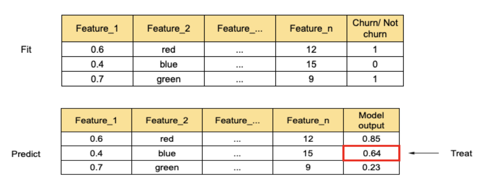
The unconditional propensity approach is based on propensity prediction and assigning treatments based on some thresholds. For example, we can train a model that predicts churn probability. Customers with a high probability (for example, higher than 0.7) can be labeled Lost causes because they have a high probability of churn and will churn anyway. Customers with a low probability (for example, lower than 0.3) can be labeled as Sure things, as they will not churn anyway.

However, we cannot differentiate between Persuadables and Do-not-disturbs and will just treat customers in the middle of the propensity score range, as illustrated in the figure below.

Direct uplift modeling

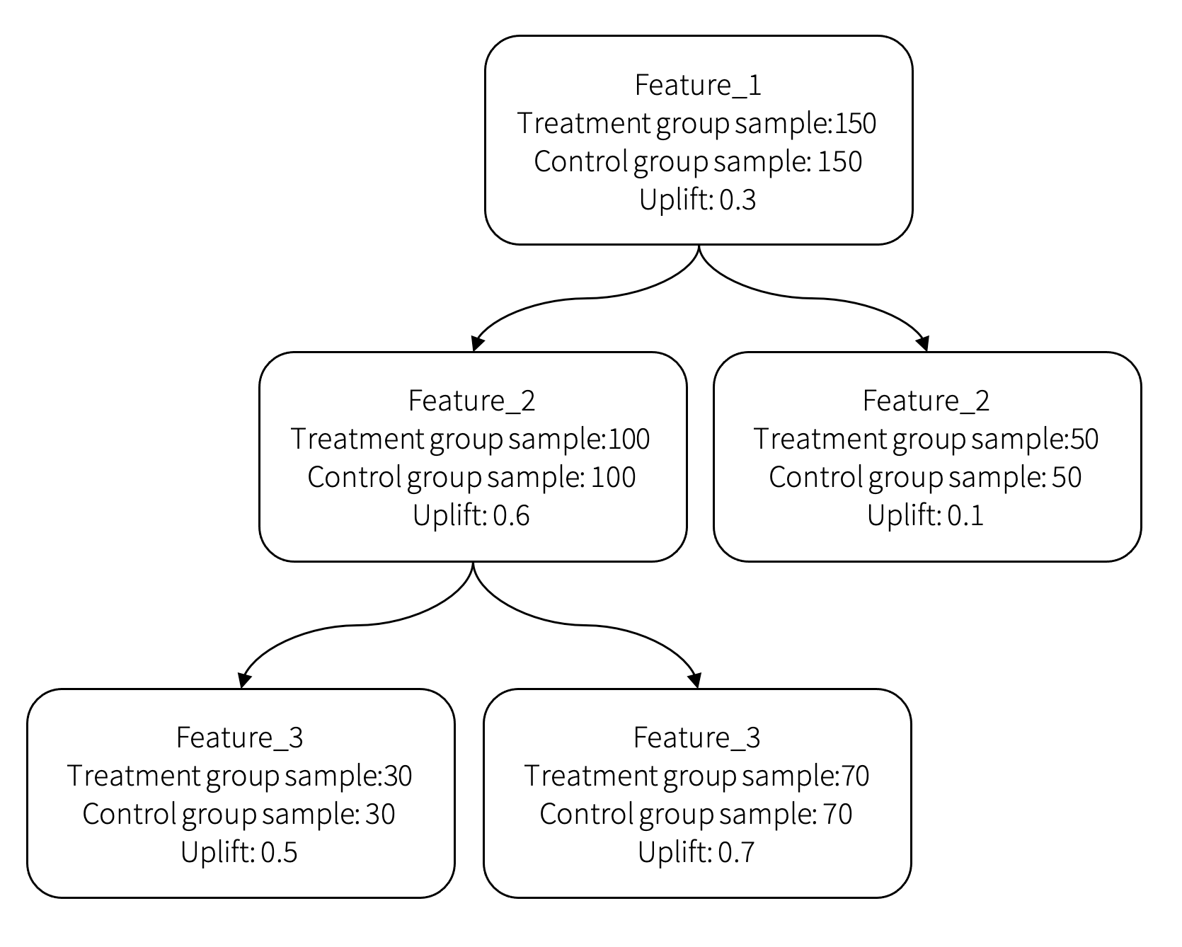
The second approach is direct uplift modeling. It can be implemented as a decision tree model with special partition criteria. For example, we can build a tree using the divergence between the distribution of the target variable in the treatment and control groups as the partition criteria. The uplift is evaluated at every leaf based on the difference between the treatment and control sample distributions in it:
$$
\text{Gain}_D = D_\text{after split}(P, Q) − D_\text{before split}(P, Q),
$$
where $P$ and $Q$ are the target variable distributions in the control and treated groups, respectively, and $D$ is the measure of divergence between the distributions. In our case, the target variable is binary—churn or not churn. Consequently, distributions $P$ and $Q$ are Bernoulli distributions, and we specify them as tuples $P = (p, 1-p)$ and $Q = (q, 1-q)$, where $p$ and $q$ are the churn probabilities for the treatment and control groups, respectively. The main divergence measures we can use are as follows:

1. Kullback–Leibler divergence:
   $$
   KL(P, Q) = \sum_{i=1}^2 p_i \log\frac{p_i}{q_i},
   $$

2. Euclidean distance:
   $$
   E(P, Q) = \sum_{i=1}^2 (p_i - q_i)^2,
   $$

3. Chi-squared divergence:
   $$
   \chi^2(P, Q) = \sum_{i=1}^2 \frac{(p_i - q_i)^2}{q_i},
   $$

where $p_i$ and $q_i$ are the elements of tuples $P$ and $Q$, respectively. An example decision tree that illustrates how customers are split into groups and how uplift is estimated for each group is shown in the figure below:

Meta-learners

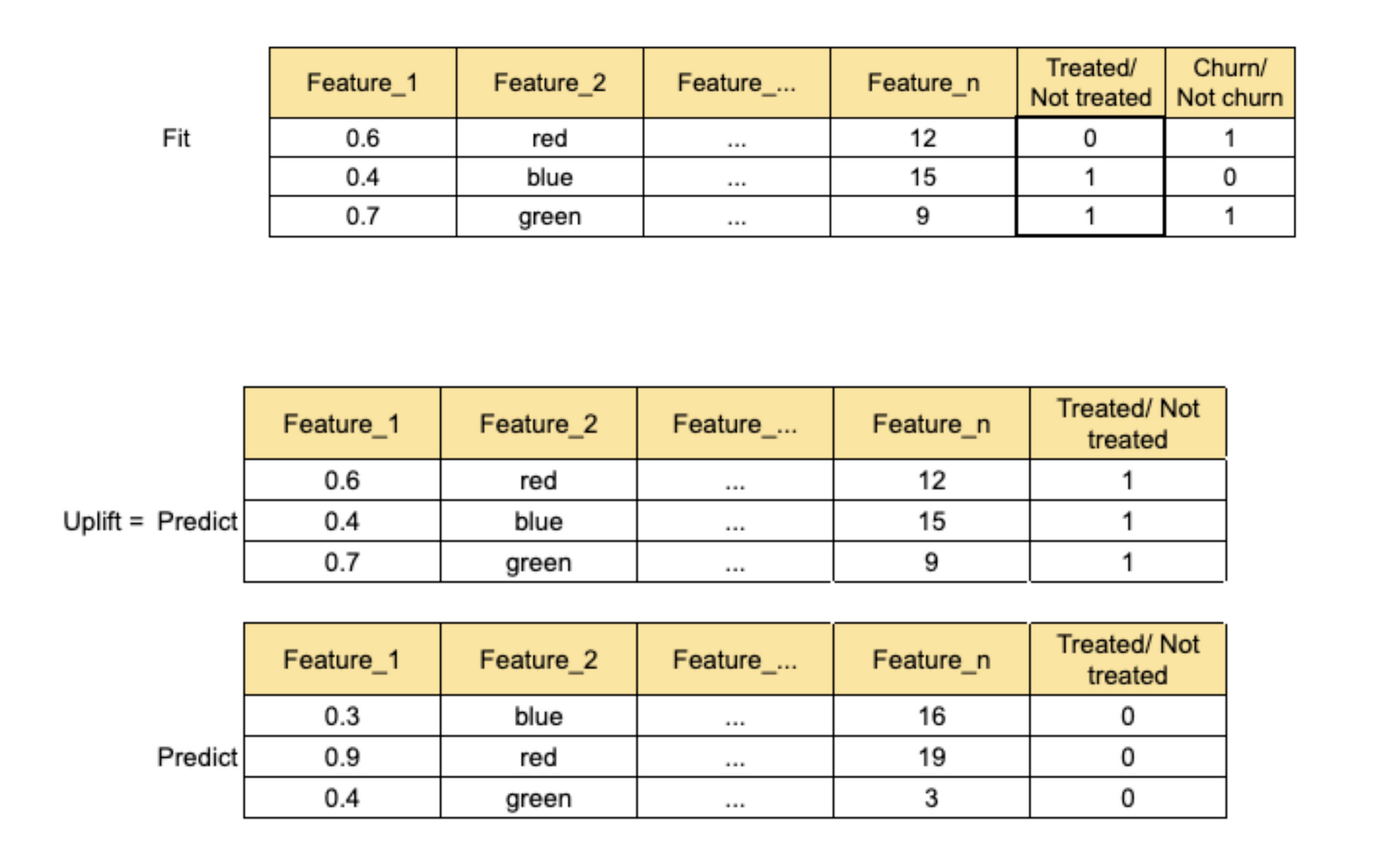
The third group of methods is collectively known as meta-learners. One possible approach, known as S-learner, can be implemented using only one classification model. The main idea is to train a model with a special binary feature that indicates whether a sample is in the treatment or the control group. The target label corresponds to churn.

We use this model to make two predictions for each profile. We first evaluate the model with the treatment feature set to 1, followed by the model evaluation with the treatment feature set to 0. The difference between the two predictions is the uplift level. This process is illustrated in the figure below.

The second way of implementing a meta-learner is known as a transformed target [2]. Instead of adding a feature that indicates whether a sample belongs to the control or the treatment group, it transforms the target value to incorporate this information.

The standard labeling notation for this method is to use 1 for a positive outcome and 0 for a negative outcome. In the case of churn, a positive outcome means that the customer stays with the company, and a negative outcome means attrition. So, we set the target labels to 0 for a churned customer and 1 for a non-churned customer.

The first step is to compute a new (transformed) target label based on the original target variable (binary churn/non-churn flag) and binary communication flag (whether the customer is in the treatment or the control group) using the following logic:
$$
z_i = \begin{cases}
1, \quad \text{if } w_i = 1 \text{ and } y_i = 1\\
1, \quad \text{if } w_i = 0 \text{ and } y_i = 0\\
0, \quad \text{otherwise}
\end{cases}
$$
where $z_i$ is the new target for customer $i$, $y_i$ is the original target for customer $i$, and $w_i$ is the treated/non-treated flag assigned to the customer. In other words, the target will be equal to 1 if the customer got the treatment and stayed or did not get the treatment and churned and will be 0 in all other cases.

The second step is to create a training sample with an equal number of customers in the treatment and control groups, that is, $p(w = 0) = p(w = 1) = 1/2$, and fit the model that outputs the probability of $z = 1$. Assuming that we have a model that estimates the probability of $z = 1$, it can be shown that the uplift can be estimated as follows [2]:
$$
\text{uplift} = 2 \times p(z = 1) - 1
$$

The third strategy, known as T-learner, involves building two independent models. One model is trained on the treated group and another on the control group. Each profile is scored using both models, and the uplift is estimated as the difference between the models.
$$
\text{uplift} = \text{score}_\text{treated} - \text{score}_\text{control}
$$

An alternative approach, known as X-learner, involves building two dependent models. It is commonly used when the treatment group is small, and we have to balance the dataset somehow. This method consists of four stages:

1. The first step is to train two models—one for the treatment group (T) and another for the control group (C) with churn/non-churn targets $y$:
   $$
   \begin{aligned}
   \text{model}^T &= \text{fit}(x_{\text{train}}^T, y_{\text{train}}^T) \\
   \text{model}^C &= \text{fit}(x_{\text{train}}^C, y_{\text{train}}^C)
   \end{aligned}
   $$

2. The second step is to make a prediction for the treatment group using the control group model and a prediction for the control group using the treatment group model:
   $$
   \begin{aligned}
   \widehat{y}^C &= \text{model}^{C.\text{predict}(x_{\text{train}}}T) \\
   \widehat{y}^T &= \text{model}^{T.\text{predict}(x_{\text{train}}}C)
   \end{aligned}
   $$

3. In the third step, the target for both models is transformed. The new treatment group target $\widetilde{D}^T$ is computed using predictions of the control group model as the difference between the real target value and the control model prediction:
   $$
   \widetilde{D}^T = y_{\text{train}}^T - \widehat{y}^C
   $$
   The new control group target $\widetilde{D}^C$ is computed using predictions of the treatment group model as the difference between the prediction of the treatment model and the real target value:
   $$
   \widetilde{D}^C = \widehat{y}^T - y_{\text{train}}^C
   $$

4. Next, we train a new set of models using the transformed targets and make predictions:
   $$
   \begin{align}
   \text{model}_\text{new}^T &= \text{fit}(x_\text{train}^T, \widetilde{D}^T)\\
   \text{model}_\text{new}^C &= \text{fit}(x_\text{train}^C, \widetilde{D}^C)\\
   \widehat{Y}_\text{new}^T &= \text{model}_\text{new}^{T.\text{predict}(x_\text{train}}T)\\
   \widehat{Y}_\text{new}^C &= \text{model}_\text{new}^{C.\text{predict}(x_\text{train}}C)
   \end{align}
   $$

5. Finally, the uplift level is estimated as a weighted sum of two model predictions:
   $$
   \text{uplift} = g \times \widehat{Y}_\text{new}^C + (1-g) \times \widehat{Y}_\text{new}^T
   $$
   The blending weight $g$ can be set to 1 if the target group is larger than the control group and 0 otherwise.

In our experience, the one-model approach proved to be a reasonable solution for most projects.

From Uplift to Next Best Action

The uplift framework enables the evaluation of specific treatments for specific customers at specific points of time. The best treatment can be determined by evaluating multiple possible actions and choosing the option that is expected to deliver the highest uplift. For example, the output of the treatment scoring procedure can look as follows:

This output can be further post-processed using business rules to filter out invalid actions or override recommendations produced by the model.

In practice, the number of possible treatments can be very high. For example, a customer retention campaign can be specified by a promotion type (buy-one-get-one, etc.), promoted product, and communication channel (email, phone call, etc.), so the number of specific treatments can be as high as the number of possible combinations of these three parameters. It is usually impossible to accurately estimate the uplift for such a large number of distinct treatments. This problem can typically be alleviated by defining 5–10 treatment types and manually creating campaign templates for each type.

Model Evaluation

The last problem we need to address is the evaluation of model quality based on historical data. This step usually precedes the A/B testing in production. We typically use several methods that help to evaluate different aspects of the model:

• Gains curves (basic check)
• Estimation of uplift accuracy at the group level
• Estimation of the uplift in deciles
• Uplift comparison

Incremental gains curve

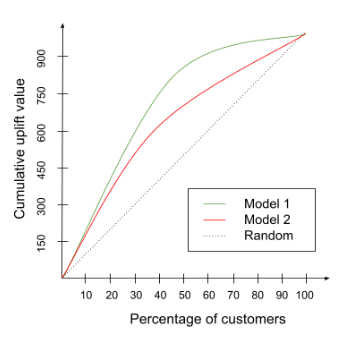
Incremental gains curves help analyze the uplift delivered by a propensity model compared with random targeting. For example, the following plot shows the percentage of churners in a sample that includes various percentages of customers. If the sample is drawn randomly, the ratio between the sample size and the number of churners is constant, and the corresponding cumulative curve is a straight line. If the sample is created by sorting customers based on the churn score produced by some reasonable model and selecting the top percentile, then the concentration of churners will be higher, at least for the top percentiles. This is the most basic validation that is not specific for uplift modeling and next best action, but it helps validate propensity models that are used as components or developed for data exploration purposes.

Uplift estimation at a group Level

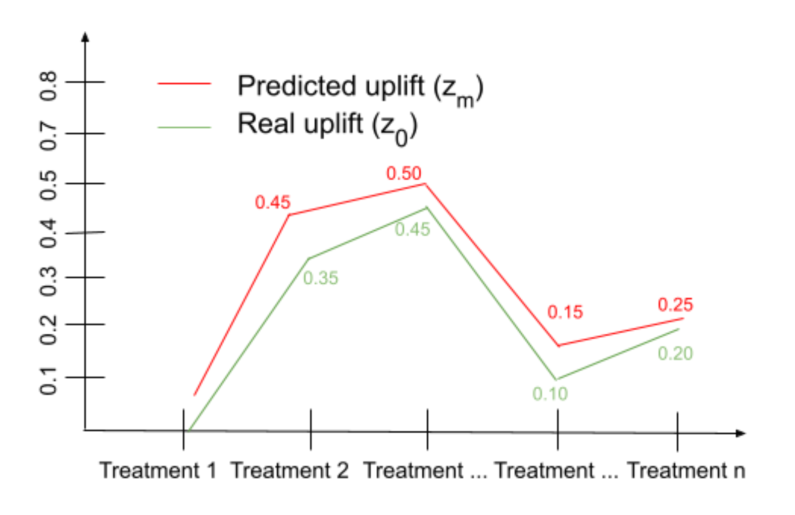
This is a business metric that allows us to evaluate how well the model performs for specific treatments or treatment groups. The idea is to estimate the churn level within every treatment group and compare the results with the churn level of the control group using the following algorithm:

1. Observe the churn rate $x$ for the treatment group and the churn rate $y$ for the control group.
2. Calculate the uplift at the group level $z_0 = x - y$.
3. Estimate the uplift based on the model output at the customer level: $z_i = p(\text{treatment})_i - p(\text{no treatment})_i$.
4. Estimate the uplift at the group level $z_m = \text{mean}(z_i)$.
5. Compare $z_0$ and $z_m$.

If the model is accurate, the curves spanned on values $z_0$ and $z_m$ over all treatments should have similar shape:

Uplift estimation by deciles

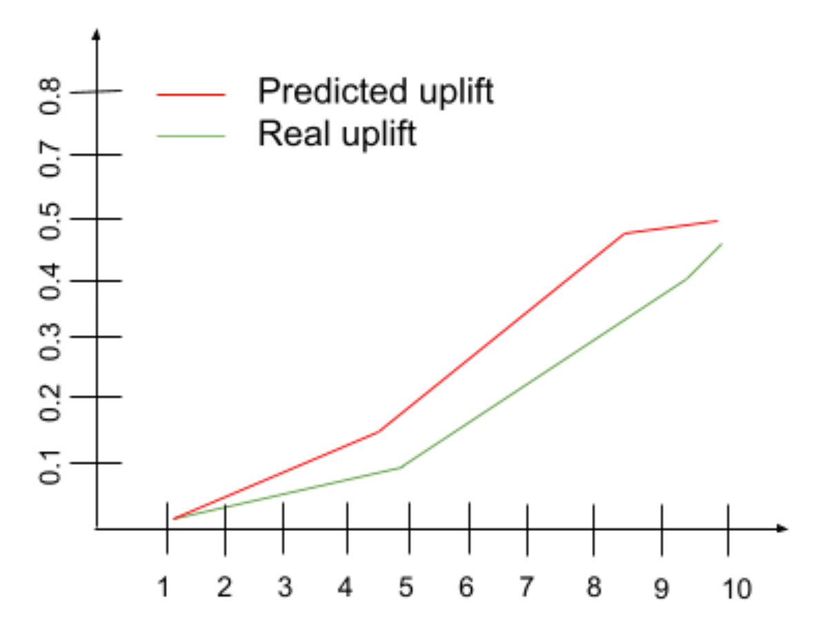
This method measures the uplift level on deciles. The first step is to sort customers by the uplift level from high to low and divide them into deciles. Within every decile, we have real control and treatment samples of both churn and non-churn, and we can estimate the difference between the churn rates in the treatment and control groups in each decile. This produces a plot similar to the figure below (for each treatment). If the model is accurate, the curves have the same shape, showing growth from the lowest decile to the highest.

Uplift for historical actions

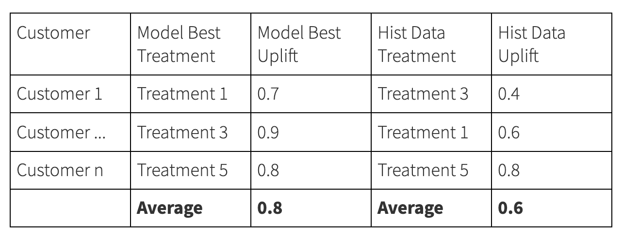
In the next best action model, we estimate the uplift for all treatments and select the treatment that is expected to deliver the highest uplift. On the other hand, we have historical data with the treatments that customers got in reality, and we can predict the uplift levels for them. So, we can estimate the average uplift level for the best predictions and real treatments and compare these two values. The predicted uplift should be higher if the model is meaningful.

Conclusions

We have described a workflow for building the next best action models. This workflow includes bias correction, propensity modeling, uplift estimation, and model evaluation steps. For each of these steps, there are many methods and techniques that provide different trade-offs in terms of complexity, restrictiveness of assumptions, and quality of results. In many practical settings, it is possible to build and, even more importantly, evaluate a reasonable next best action solution using relatively basic methods and limited access to marketing resources.

References

1. Heckman, James (1974). “Shadow prices, market wages, and labor supply”. Econometrica. 42(4): 679–694.
2. Maciej Jaskowski and Szymon Jaroszewicz (2012). “Uplift modeling for clinical trial data”. ICML Workshop on Clinical Data Analysis.
3. Austin, Peter (2014). “The use of propensity score methods with survival or time-to-event outcomes: reporting measures of effect similar to those used in randomized experiments”. Stat Med. 33(7):1242-1258.