Retail price modeling for replenishable and seasonal products

Pricing is one of the key factors that drives a successful retail business model, and it is also one of the most difficult to manage. Retailers made lots of improvements on their pricing strategies over the last decade, moving from cost plus or value pricing to modern day AI-driven price management. In this article, we will discuss the common process with which retailers set their pricing, the challenges that they are facing in the area of price management, and how they incorporate big data analytics and machine learning into their pricing strategy.

1. The retail pricing process

Retail has a complicated pricing process that involves almost all of the functions in the retail company - from Finance, Merchandising, and Inventory Management to Pricing, Marketing and Store Operations. We start with a high-level description of this process to set the stage for further discussion of pricing models, and then explain how price modeling fits into the big picture and helps to improve retail profitability.

1.1 Plan-to-sell process

A common practice of the retail pricing process is to start by setting up a strategic or financial goal. The financial goal is usually based on historical data, for example, a 5% increase of year over year sales and margin, or $20 billion sales and $8 billion in margin. Once the goal has been set, multiple teams build a plan to help achieve that goal. This process, known as the plan-to-sell process, is led by a merchant team, with Assortment Planning, Inventory, Pricing and Marketing teams helping the merchants manage their respective processes and achieve the financial goal, as illustrated in Figure 1.

Figure 1. An overview of the plan-to-sell process.

The plan-to-sell process is generally focused on developing two groups of assets: a Buy Plan that specifies what to buy, and a pricing plan and models that specify how to sell, as shown in Figure 2.

Figure 2. Assets developed in the scope of the plan-to-sell process.

The plan-to-sell process starts with development of a Buy Plan by the merchandising team. This plan typically includes the following:

• Composition of the buy: What items do we want to carry in our stores? Size, color, and all other attributes, including a price banding for each program (program is a set of SKUs, e.g Levis Boys Jeans of different fit, style, color, and size can be a program).
• Size of the buy: How many units do we need for each item/program/category?
• Lifecycle of the buy: Usually only applies to seasonal items.

Once the merchant team has established the initial buying strategy, the pricing plan can be developed to specify how the merchandise will be sold. This step is known as pricing optimization planning, and we describe it in more detail in the next section.

1.2 Price optimization planning

Price optimization planning aims to create a high-level pricing strategy, and it often uses rougher pricing models. The actual price setting is done later at the selling stage using more fine-grained and accurate pricing models.

Just like any optimization problem, price optimization planning requires the definition of target metrics that need to be maximized, variables that can be changed to maximize the target metrics, and constraints that have to be taken into account as we search for optimal values of the variables. For most retail companies, these aspects of the price optimization planning look as follows:

• Variables. The structure of retail pricing starts with cost, and the listed retail price or regular price is obtained by adding a markup to the cost. Promotional offers or markdowns can be applied on top of the regular price to obtain the selling price, also known as out-the-door (OTD) price. Price optimization can focus on regular prices or OTD prices, depending on the price communication strategy (everyday low pricing or high-low pricing). Without loss of generality, we will assume that the goal of price optimization is to optimally adjust the OTD price, and that these price adjustments are communicated to customers via promotions and discounts.
• Metrics and objectives. The fundamental goal of price optimization is to maximize profits. However, the exact metric to be optimized can differ across different product types. For replenishable items, since inventory can be replenished and there are no constraints for the inventory ownership, the goal is to optimize profit for every selling period. For seasonal items, because the inventory is limited and fixed, the goal is to maximize sales for the entire item life cycle.
• Constraints. Price optimization can be constrained by the available inventory, as well as retailer’s pricing rules and policies. For price optimization planning purposes, it is typically assumed that the inventory will match the sales goals.

The price optimization planning usually starts with the following input data:

• Sales history and trend
• Cost components
• Promotion and events
• Elasticity of demand estimated with sales data
• Product and store attributes
• Seasonality and holiday impact
• Competitive pricing

These inputs are used to roughly estimate optimal pricing parameters. The pricing models used at this stage are pretty high-level: they usually stay at category level (i.e. use the average price elasticity of the entire category) of the entire geographic location, and assume that the available inventory will be enough to achieve the sell-through goal in the plan. The pricing model uses historical sales data to calculate the own-item price elasticities of demand, and assumes elasticities are constant with no geolocation adjustment or price discount adjustment. Or in other words, elasticity for one particular item will remain the same no matter whether you are selling it in a store in Hawaii or Alaska, or whether the price is 20% off or 80% off. For cross-item effects, competitor pricing is adjusted on an ad-hoc approach if necessary. For example, a private label fashion dresses will not have cross-item effects and competitor price effects since every category of dresses is not the same, and a private label is only carried in one retail brand. But for brand name jeans, like Levis, some ad-hoc adjustment is necessary.

The output of the pricing model run is a complete pricing plan that optimizes the pricing strategy of the product over an entire life cycle. A plan for seasonal products will include both an in-season promotion pricing plan and a post-season clearance markdown pricing, as the pricing goal for the seasonal plan is to achieve maximum sales revenues for the entire item life cycle or entire season. A plan for replenishable items is usually much simpler since it aims to maximize margin in each selling period.

This pricing plan will also get fed back to the Buy Plan to adjust the size of the buy. For example, if the original Buy Plan does not have enough unit buy to achieve the financial goal after exhausting all the pricing options, then that information needs to feed back to the Buy Plan for increasing the unit buy.

2. Challenges of the retail pricing process

The previously described plan-to-sell model that is currently used in most retail businesses is more of a strategy and people-driven process than a data and technology-driven process. The lack of predictive analytics, gaps in process automation, and the limitations of price management systems can and often do significantly decrease pricing efficiency -- and eventually harm profits. In this section, we describe several typical examples of such issues.

2.1 Inaccurate forecasting and lost sales

Price planning often uses simple demand models, so that the forecasting is based on trends. In other words, the plan-to-sell model looks at what we sold in the past and estimates future demand based on these sales numbers.

One of the most common issues with this approach is that lost sales are ignored in these estimates. The true level of demand is a sum of actual sales and lost sales, so a demand forecast that relies solely on sales number and does not account for lost sales is not accurate. This issue can be alleviated by using more advanced demand models that account for inventory and estimate true demand.

2.2 Inaccurate modeling of the demand heterogeneity

The second challenge is that pricing planning modeling typically stays at too high a level, although it uses different techniques for seasonal and replenishable items. It often assumes constant elasticity and assumes that all geo locations have the same selling pattern and trend. It also assumes no inventory constraints, which is definitely not true, especially for seasonal items.

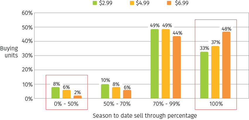
One common issue with this approach is that models with high level of aggregation cannot properly account for demand heterogeneity. For instance, Figure 3 shows a real-life example of a season-to-date sell-through chart for three price bands ($2.99, $4.99, and $6.99). There are four sell-through percentage groups in the chart (less than 50% of units sold, 50% to 70% of units sold, 70% to 99% of units sold out, and 100% sold out or out of stock), and each bar shows the percentage of purchased merchandise (in terms of SKUs) in the given price band that fall into the corresponding sell-through bucket. For context, the chart shows the situation on the 30th week of sales for a product with a life cycle of 40 weeks.

As you can tell for the $6.99 priced items, 48% of total purchased inventory units are sold out in their geolocations, while only 2% of units sold less than 50%. Given that this is a snapshot of the situation at the end of product life cycle, it tells us that we priced too low for those sold out locations, and priced too high for the low sell-through areas. Therefore, if we price all store locations with the same discount, we would leave lots of money on the table.

Figure 3. A real-life example of sell-through rates variation.

In order to resolve this issue, we have to go to a very granular level to build our pricing model, and feed the model with real time inventory and selling data to make the price recommendation more optimal. The level that a retailer can use to run the pricing model depends on the price execution limit. For example, if Levi’s Boys Jeans are displayed on the same fixture, then the model can only pick one price for the entire program by store. If Ninja Blenders have one facing for each model on the shelf, then the model can price those blenders at the item/store level. How frequently the retailer can update the model depends on the size of the data set, IT resources, advertising frequency and price change labor in the stores. It typically runs once a week, while online store pricing can run much more frequently.

2.3 Operational challenges

Advanced modeling techniques can help resolve issues with unaccounted lost sales and heterogeneity of demand, but there are other challenges that lead to suboptimal pricing which are very difficult or impossible to resolve by just improving the pricing model.

For example, a seasonal buy usually has a long lead time. It often takes one year from planning the buy until you can start selling the products. Such a long lead time frequently results in not buying enough units in certain areas. Inventory allocation is another challenging task to get done just right, as retailers always end up not having enough inventory in certain stores, but too much in others. Retailers also face other operational challenges which constrain the price optimization, such as store execution and advertising execution. They wish that they can use real time pricing to change prices several times a day, but this would cost too much store labor and would be confusing for customers. Retailers also wish that they could have different versions of advertising by store clusters or geo locations, but it costs too much to alter advertising with such multiple versions.

In the retail world, “pricing touches everything, and everything touches pricing”. Price management creates cross-functional chaos, so a price solution that addresses only pricing itself will not work for a retailer. That is one of the key reasons why most of the off-the-shelf price management software does not work well in the complex retail environment.

3. Basic price modeling

In the previous two sections, we outlined the context in which retail price modeling and optimization happens, and described how it relates to some other enterprise processes. In the remainder of this article, we drill down into the mathematical details of price modeling. We introduce several basic methods and techniques in this section, and then develop more specialized methods separately for replenishable and seasonal products in the subsequent sections.

3.1 Linear demand model

The most basic price optimization model can be defined using the following simple equation that ties together an item’s cost, demand, price, and profit:

In order to evaluate the basic profit equation for a given price, one needs to specify and estimate the demand function that quantifies the dependency between price and demand. The most basic choice for the demand model is a constant-elasticity model, also referenced to as a loglinear or simply linear demand model. This model is based on the assumption that the demand decreases by a fixed percentage in response to each percent of price increase:

where elasticity is a coefficient with an estimate based on the sales data. Given that this coefficient and current demand are known, one can straightforwardly evaluate price increase and decrease scenarios using the basic profit equation above (by changing the price by a certain percentage and demand by the same percentage times elasticity). It can also be shown that the constant elasticity assumption is equivalent to the following relationship which we will use later in this article:

In the coming sections we will discuss the limitations and trade-offs of this simplistic model, as well as processes needed to apply it in practice.

3.2 Limitations of the linear model

The linear demand model uses sales history and price change history data to estimate price elasticity, and assumes that price is the only factor that drives demand change. The linear model is typically appropriate for the pricing planning stage, since the level of the planning stays at the category level. This has enough data to normalize the demand and to not have much impact on cannibalization and affinity. But once the retailer passes the planning stage and goes into the selling stage, a linear demand model will not be enough to catch all the moving pieces, since pricing is not the only parameter to impact the demand. The following parameters also need to be considered in the comprehensive modeling process:

• Promotions and events. Retailers use multiple traditional marketing and digital marketing channels to promote their products. They also use different kinds of offers to get to optimal prices, such as percent-off offers, buy one get one free, coupons, stacking offers, etc. It is important to figure out the promotion lift by marketing channel and offer type, since they have different impacts on the promotion lift. For example, selling the same Barbie doll for $20 via an ad vs. $20 not via an ad would yield different units.
• Price perception and competitive pricing. Some items are highly price sensitive, while others are not. For example, everybody knows how much detergent from Tide should cost, but very few people know how much a private labor cocktail dresses should cost.
• Cannibalization and affinity. When one item has been promoted, negative demand effects cross items, and positive demand effects attached items.
• Seasonality. The demand for certain items has seasonal trends that need to be incorporated into the models for accurate forecasting.
• Volume impact. The linear demand model works well when the data has been normalized, or in other words, when every geo-product sells the same. But when the selling pattern is different by time period or by location, the model accuracy will not be very good.
• Store attributes. Elasticity will be different in different stores, depending on the demographic of those stores and their distance from competitors.
• Out of stock or size breakage. If you are running out of stock or desirable sizes in the selected location, no matter how low the price is, the unit lift just will not be the same.
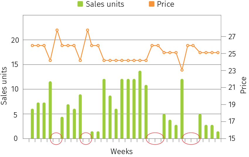
• Zero sales. The traditional linear demand modeling ignores weeks with zero sales, biasing estimates of price sensitivity. Consider a sales chart example in Figure 4. The prices in this chart are the listed promo prices for a certain product, which go up and down by week depending on how a retailer promotes this product, and sales units which represent the actual sold units. The circled weeks are the cases when this store had zero sales after a price increase. Traditional models would remove both the unit and price change history for zero sales, which (1) biases elasticity estimates toward appearing less price sensitive, and (2) optimizes prices based on these flawed estimates.

Figure 4. A real-life example of zero sales caused by a price increase.

We will discuss how these various factors can be incorporated into the pricing process in the following sections, which are dedicated to replenishable and seasonal items.

3.3 Choosing the level of aggregation

There is always a trade-off in terms of which level of aggregation the retailer picks to run the pricing model. There are two dimensions of level aggregation. One is at the geolocation level, from one store all the way to all of the store locations. The other is at the merchandise hierarchy level, from one kids apparel item with a specific size, color and style all the way to the entire Kids department. Inventory sell-through and elasticity work better if you go down to the granular level like item/store, since the elasticity is different from one store to the other, and from one item to a group of items.

Most importantly, the inventory sell-through percentage also varies from one store to the other, even with the exact same item. From example, the same down coat could be sold down to 1 in the Chicago store vs. still have 10 left in the Nashville store. Obviously, we need to price these two stores differently to maximize the margin. However, the lower level data always come with tons of noise and outliers. The goal is to find the correct aggregation level that gets the outputs most closely fit to the actual demand curve. There are multiple ways that retailer uses to resolve this issue, but the simplest way is just to move up the aggregation level. If the item/store can not yield a good fit, then we would just move to an item/store group level for aggregation. Or, if that doesn’t work, we can move up to the item/climate zone level. The best way to resolve this is to use machine learning techniques to get rid off the noise and outliers in the data, and find the nearest neighbor that provides better approximation to the actual patterns of demand.

3.4 Modeling and optimization workflow

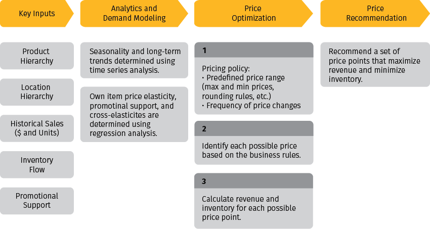
The traditional retail price modeling workflow has two parts: analytics, and optimization. Analytics use historical data to develop a baseline forecast – what would happen if we take no pricing action and just sell everything at regular prices. As we discussed in the previous sections, this forecast can be created using very basic demand models for preliminary planning purposes, and then refined using more advanced techniques to incorporate seasonality, promotional support, and cross-item effects. The forecasting model quantifies the dependency between the demand/profit and price, and thus enables what-if analysis of different pricing scenarios.

Optimization is the process that runs every possible combination of prices for every available price change date by allowed geo-product combination, and then chooses the option that provides the most revenue, or the margin which meets the business objectives and constraints. This process also estimates the amount of inventory needed to fulfill the demand at the recommended price. This price modeling workflow is summarized in Figure 5.

Figure 5. A price modeling workflow.

3.5 Model diagnostics

Optimal pricing from the pricing model generates millions of dollars in profit for retail companies. Therefore, it is very important to make sure the pricing model is recommending the correct price to maximize the profit.

The common way to diagnose the pricing model health is by running a hold out forecast. In this approach, one runs the model to forecast sales for the previous couple of weeks using its recommended prices, and then compares the forecasted sales with the actual sales to see how big the difference is. The hold out forecast usually forecasts both inventory constrained sales and unconstrained sales, then uses the mean absolute percentage error (MAPE) to measure the difference between the forecast and actual numbers. The acceptable MAPE ranges from 0% to 30%. If the error is above 30%, then the model setting should be changed, and the hold out forecast should be re-ran until the MAPE comes down to the acceptable level. This self-learning process can be automated to improve the efficiency.

It can also be the case that the model performs well on average and achieves good MAPE, but has large prediction errors (outliers) for certain products or dates. This issue can be mitigated by running hold out forecast at a very granular level, both in terms of product hierarchy and time.

4. Pricing model for replenishable items

The basic pricing model described in the previous section is acceptable for preliminary planning, but the actual price optimization for the selling phase requires the development of more accurate models that incorporate a larger set of signals and effects. These more advanced models are typically more specialized as well, as they are built for specific product categories. The first such specialization we will consider is a pricing model for replenishable items.

The best approach to pricing replenishable items is to combine machine learning and decision automation with human inputs. Modern day machine modeling helps to process big data, but it also leverages human inputs, and has governance of business rules. Additionally, it enables the input of clean attributes of the products, which is critical: the model output will not be useful without good product attributes. Business rules also act as a guardrail to the pricing model outputs, helping to prevent erroneous decisions and keep micro-decisions consistent with the overall strategy.

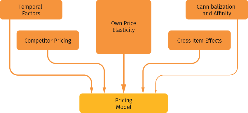
The pricing model for replenishable items has to account for several factors that are summarized in Figure 6. Own price elasticity is the most important effect in the pricing modeling, and the other effects are secondary. Cannibalization and affinity is usually the least relevant for pricing among all the secondary effects. We will further discuss below how these different effects can be quantified and incorporated into the optimization model.

Figure 6. The main factors and effects that need to be accounted for in a pricing model for replenishable items.

4.1 Own item elasticity vs. cross item elasticity

Own item price elasticity is the effect of price changes of a focal product on the sales of a focal product. Cross item effects or a comparable product index are the effects of price changes of other products on the sales of a focal product. Simultaneously modeling all own- and cross-item effects in a single, comprehensive demand model is the best way to price basic replenishable items.

The cross effects between multiple items that share similar product attributes can estimated by running a linear regression. In this case, the cross elasticity will be quantified by a regression coefficient for the price of one item in the demand model for another item. Figure 7 shows an example of cross-elasticity analysis for four similar items in the coffee maker category. In this example, private label coffee maker pricing may be a lever for moving branded items, because customers appear to trade into/out of branded items as similar private label coffee maker prices rise/fall. However, the opposite is not true, and the demand for private label coffee makers is relatively insensitive to branded prices.

Figure 7. A real-life example of cross elasticity analysis for four similar items in the coffee maker category.

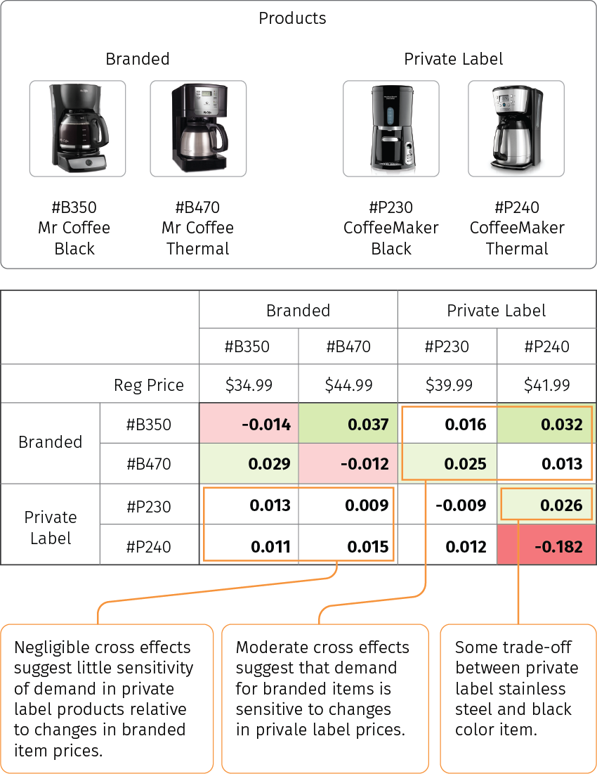
The example in Figure 7 can be extended for an arbitrary number of items, but retailers typically avoid carrying a large number of similar items that have a cannibalization impact on each other, as an over-assortment of merchandise can be a big hit to margins. In the coffee maker example, you might see a retailer carrying 20 different coffee makers, but not all those 20 items will have a cannibalization impact from each other. For instance, a $20 coffee maker will not compete with a $600 one.

4.2 Competitive pricing

A competitive pricing strategy is not all about web scraping, price matching, and undercutting competitor prices. Otherwise, a retailer would end up with the everyday lowest price on the market, which is a big margin hit, and something that most retail companies would not be able to afford. Competitive pricing is about setting the price based on what the competition is charging, and using the competition’s prices as one of the pricing model parameters to determine the optimal prices. The following two steps are what retailers often use to incorporate the competition prices into the pricing modeling.

First, a retailer runs analytics to figure out the impact from competitor’s prices on their own sales. In order to run the correct analysis, retailers need to have a thorough study not only on its internal company data, but also on competitors’ activities (such as pricing, promo etc.). It is also very important to have a profound knowledge of the market and the retailer’s position in it. This analysis needs to combine human knowledge and machine knowledge, and is a combined effort from multiple teams within the retailer. Merchants know their products best, so they can list the items that they feel are important to stay competitive on the market. The marketing team understands who their competitors are in each specific category, so they can provide knowledge on what other retailers their own customers also shop at, and work with 3rd party marketing data providers to get the detail pricing promo activities from their competitors. The pricing/data science team can use this information to run models and quantify the exact impact from the competition to the retailer’s own sales.

The impact from the competition to own sales is generally quantified using the cross item price elasticity analysis that we discussed in the previous section, but with regard to competitor’s prices:

If the cross elasticity is positive, that means we need to consider the competitive pricing when we price our own items. Since our own sales units reduce when a competitor reduces their prices, our own sales increase when a competitor increases their prices. Competitive price cross elasticity can be measured at the individual item level or with a group of items. The level of measurement is defined by the business rules, and depends on how competitors are promoting their items. For example, if retailers usually promo their underwear products by brand with multiple items during the back to school season (like all Hanes underwear being on sale for one week), then the competitor analysis needs to be done at the brand level instead of the individual item level.

The second step is to generate operational pricing rules based on the cross elasticity parameters estimated in the previous step. Once retailers have figured out the exact impact from competitors, they will add business rules in the modeling section to guardrail the model price outputs. For example, let’s look at one $79.99 brand name toast oven. If there is no impact on our own sales as long as we stay at +10% of the competitor prices in the New York market, and +6% of Chicago market, then a corresponding business rule should be added to the modeling section of this item.

4.3 Cannibalization, affinity, and pull-forward sales

The last group of effects that are commonly incorporated into the model are the effects related to demand redistribution between products, or between current and future time periods.

Cannibalization usually happens within the same category for two or more competing items when those items share lots of similar product attributes, but differ by one or few other attributes, like brand, color, flavor, price banding, etc. As cannibalization happens within the same category, we need to run the analysis on the sales of the entire category to determine the cannibalization from one item to the rest of the similar items (i.e. we calculate the total category sales change with each item price change). Normally, when you put the brand name item on promo sales, the cannibalization is much higher than when you put an unknown/private label brand on sales for these two reasons:

1. Brand name items have much high customer loyalty.
2. Brand name items are more expensive than similar items that are private label, so once they are on sale, the price difference gets smaller. Therefore, customers are more willing to trade up.

The affinity or halo effect occurs when promoting one item has a positive influence on other items. For example when you promote grills, grill accessories will also get a sales lift. Or, when you promo Coke, you might see more sales from other snacks. A basket analysis will be able to determine the affinity and halo effect. We need to look at historical transactional data across multiple promotional periods, analyze all baskets that contained the item promoted, and determine among all those baskets which were the common items that were not on promotion. What you should get is finding that something like 50% of grill baskets had a grill accessories purchase. Since grill accessories were not promoted, any lift we see in sales to grill accessories during that promotional period can be attributed as an affinity to grill. This information is vital, as it allows us to determine the affinity effect of the promotion at the same time. This informs us to not price down correlated items at the same time, as we would be giving up margin unnecessarily.

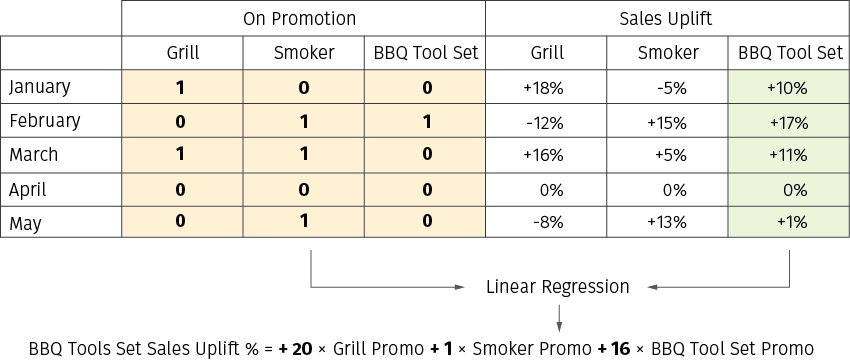
In practice, a retailer can run multiple promotions at the same time, so that there is a complex interplay between multiple affinity effects. A retailer can use regression analysis to disentangle this mix and isolate the effect for an individual promotion. Consider an example data set in Figure 8: it includes sales and promotion data for three products over five months. The impact of each promotion is quantified using single-output or multi-output regression analysis where promotion flags are inputs, and sales uplifts are the target label.

Figure 8. An example data set for affinity effects analysis. Sales uplift is the change in the number of baskets with a given product compared to the baseline forecast.

The pull-forward effect, also known as the pantry load effect, only happens in consumable categories. The pull-forward effect occurs when consumers see a commodity they regularly purchase, which has a long shelf life (e.g. bathroom tissue, detergent), go on promotion. When the item goes on promotion, the customers tend to buy a significantly larger volume than they usually purchase. They stock-up on the product for a period of time, and therefore will not buy the item at their regular frequency until they are out of stock.

To calculate pull-forward, you first need to determine the baseline purchase frequency of those items, then look at historical promotional data, and determine the effect on sales post promotion. So, if an item was promoted for a month, and if the baseline purchase frequency for this item is purchased every 3 months by the consumer, and it has a 4 month shelf life, one would look at 4 month of sales data past the promotional date to see whether the item’s weekly sales are below the baseline. If it is below, it would be considered a pull-forward effect, provided another item in the category is not promoted and did not record a lift. One needs to consider pull-forward as an impact not only to item sales, but also to category sales, as the promoted item that is being stocked by the consumer can impact the overall category performance for a period of time too.

For a replenishable item, since the inventory is unconstrained, the following relationship is generally true:

4.4 Price optimization for replenishable items

It seems challenging for retailers to combine all the above factors together into pricing modeling for replenishable items -- so how do they do it? This process takes two steps:

1. Run historical data to calculate own item elasticity and figure out the relationship between items. The output of this step is a set of parameters that quantify which item sets will cannibalize each other or have affinity for one another, what the cross elasticity is between items, which items will be impacted by competitor pricing, and by how much.
2. Run what-if analysis for all possible price change scenarios, and find the scenario that will yield the highest total sales/margin for the items set.

Let us consider an example shown in Figure 9. The historical data analysis found that when item A (Tostitos Chips) go on sale, item B (Crunchy Cheetos) sales will go down (cannibalization), but item C (Tostitos Salsa) sales will increase (halo). Additionally, item A has a pull forward sales impact for two months, so items A+B+C+(A pull forward) will be combined as an item set for the price model run.

Figure 9. An example of price optimization for a replenishable item that combines multiple effects together. What-if analysis is done for two scenarios for Item A - Price 1 ($3.00) and Price 2 ($2.50).

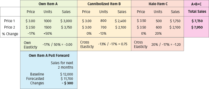
In the above example, the sales difference between Price 1 and Price 2 is $7950-$7150-$300 = $500, and hence Price 2 (a promotional price of $2.50 for item A) is a good price recommendation.

Retailers typically do not directly dial competitor pricing into price modeling. Instead, they use it as a business rule to guardrail the price change choices in the what-if analysis above. For example, if the historical data analysis shows that the sales impact is negative once we priced +10% or more to our competitor pricing, we would cap our price choices for the what-if model at +10% of our competitor’s prices.

An alternative approach to the optimization process described above is building a high-capacity predictive model (using methods like boosted decision trees or neural networks) that uses the coefficients estimated by econometric models (cannibalization, halo, etc.) and other signals as features, and forecasts profits or revenues. This approach is more flexible and accurate given that the outputs of econometric models are combined with sales time series data, inventory data, and other features that help to improve demand forecasting.

5. Pricing model for seasonal items

A pricing model for seasonal items is different than that for replenishable items for a couple reasons. First of all, seasonal buy has a long lead time, inventory is committed, and there is not much flexibility to adjust the inventory quantity after the purchase. Therefore, as retailers always consider seasonal items to have sunk costs, the goal for pricing the seasonal items is to maximize revenue instead of margin or profit. This can be illustrated by the following toy example. Consider a retailer that has two units of some product in stock, and the cost of each unit is $10. Compare the following two scenarios: a retailer sets the unit price to $15 and sells both units by the end of the season, or sets the unit price to $30, manages to sell just one unit, and throws away the second one. In these two scenarios, the margins are different ($5 and $20, respectively), but revenues and total profits will be the same, $30 and $10, respectively.

Second, seasonal items have a much shorter life cycle than the replenishable items. For example, most of the winter goods usually get delivered to stores in late October, go on clearance after Christmas, and liquidate in March to free up store space for spring goods. Therefore, the life cycle for winter goods only lasts for five months, with a peak selling period of two months. Thus, it is more challenging for retailers to price seasonal items than replenishable items.

5.1 Seasonality

Seasonality is the most important parameter for the seasonal pricing model. Seasonality usually consists of periodic, repetitive patterns in demand, usually caused by weather or holidays. For example, the winter seasonal goods uplift is caused by cold winter weather, and the Christmas season uplift is caused by the holiday of Christmas. Seasonality does not include non-recurring events that impact demand, such as snow storms, hurricanes, marketing promotion events, etc. It also does not include price-driven changes in demand.

Retailers usually estimate seasonality at the national level when they are in the planning stage to compose the seasonal buy, and go down to the climate zone level when they are selling the products. Season code and sub season code are other key product attributes that retailers use to estimate seasonality. For example, fall is one season code, and has three different sub season codes: the regular fall sub season; back to school sub season, and Halloween sub season. The demand of regular fall sub season goods is driven by weather, and depends on how cold or how early winter comes. Back to school demand is driven by the date that schools open in the area. Halloween is a floating holiday, so the demand for Halloween goods changes based on the actual day of the week that Halloween falls on every year. As you can tell, although all three sub seasons belong to the fall season code, the seasonality of them varies drastically. Therefore, it is important to estimate the seasonality by the sub season code.

In statistics, there exist a large number of methods for seasonality detection, measurement, and adjustment (i.e. removal of the seasonality components). In the next two sections, we discuss two relatively basic techniques for seasonality measurement that are known to be efficient for retail pricing applications. Both techniques are based on the nearest neighbor approach - they try to estimate the future seasonality trend by finding a sample in historical data that is similar to the current situation. The difference between them is how the similarity (distance) metric is defined.

5.2 Seasonality estimation using the difference between time series

The first method we consider uses the correlation between time series as a distance metric to find a historical sample similar to the current situation, and estimate the seasonality uplift for the next month(s) from it. The methodology is as follows:

1. Pull 3-4 years of historical data for weekly sales units and revenues at promo prices or regular prices for a given climate zone and program.
2. Use elasticity to remove the price impact. This can be done based on the definition of the constant-elasticity demand function provided in the beginning of the article:

3. Find the most similar weekly sales pattern in the previous years using the correlation coefficient between time series as a similarity metric, and use that year’s sales pattern to forecast the seasonality of the current year.

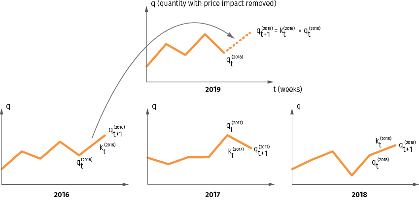
For example, in order to find the seasonality of Feb 2019 for winter season coded items, you need to run the correlations of week-over-week sales unit changes from Oct 2018 to Jan 2019 versus the previous 4 year weekly sales unit changes during the same period, and find the year that best fits the same pattern as the current year. If the 2016 winter season selling pattern is the best fit, then you would use Feb 2016 to estimate Feb 2019’s seasonality multiplier (uplift). This example is illustrated in Figure 10.

Figure 10. Seasonality estimation using nearest neighbor search in time domain. The sales quantity for week t is denoted as qt and the seasonality multiplier is denoted as kt

5.3 Seasonality estimation using a custom distance metric

Ideally, the seasonality computation should be done at the climate zone, sub season code, and program level (e.g. tropical area, sub season back to school, and Disney character boys t-shirt respectively). Unfortunately, it is not always possible to find a historical sample that is highly correlated with the current situation for a given climate zone and program, as the number of samples is limited by just the past 3-4 years. At the same time, one can argue that it makes sense to not only look at the past samples for a given pair of climate zone and program, but also at related or similar zones, sub seasons, and programs. This idea essentially means that we can introduce a more elaborated distance metric that accounts not only for correlation between time series, but also for distances between sub seasons and programs. Once this metric is defined, we can search for a nearest neighbor in a larger set of samples to find the seasonality multiplier.

Let us consider an example illustrated in Figure 11. We define the distance metric between two samples as the distance between a two-dimensional vector. The first element of this vector is the sub season numerical code. The codes are assigned to sub seasons sequentially, so the difference between the codes naturally quantifies the temporal distance between the sub seasons. The second element of the vector is defined as the average seasonality multiplier (month-over-month sales change) for the past three months. These two values are computed for all sub seasons and programs, and thus each pair of a sub season and program is mapped to a point in two-dimensional space. We then search for the nearest neighbor in this space and estimate the seasonality multiplier for the next time period based on this sample. Dissimilar to the time series correlation method described in the previous section, the sample may or may not belong to the same sub season or program.

Figure 11. Seasonality estimation using a distance metric with sub season and program components.

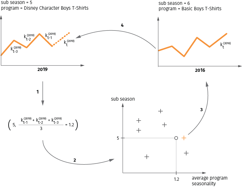
The nearest neighbor analysis with custom distance metrics is very useful for seasonal pricing modeling. Retailers purchase most of their seasonal items once a year, and as they usually add new products or new categories to new store locations to expand their business, it is difficult to find meaningful data in the historical data set. The nearest neighbor analysis helps to solve this problem.

5.4 Dog and winner approach (slow seller vs. quick seller)

As we mentioned before, seasonal items have a short selling window with a fixed amount of inventory units. Therefore, the goal for pricing the seasonal items is to maximize the sales for the entire life cycle instead of maximizing the sales/profit for every single transaction. If we are running out of stock before the season ends, that means we priced too low and left money on the table. If we are selling too slowly, that means we priced too high and will lose money in the end due to a high leftover inventory that will be sold below cost after the season.

It is very important to differentiate slow sellers (dogs) from quick sellers (winners), and price them differently. Typically, dogs remain dogs and winners remain winners for the entire season, since the reason for a dog is due to the product itself, like a color, style, or fit that is less appealing to customers. It is not due to the weather or any other outside reasons. Therefore, identifying the dogs in the early season will help retailers address the problematic items earlier, and avoid a margin loss post-season.

The most important metric to identify dogs is the sell-through rate, but we should not use a straight sell-through category rate because it varies across locations and products. For example, although a lightweight jacket and a heavy winter coat belong to the same outerwear category, their demand curve is absolutely different during the entire season by different locations. A good methodology to identify the dogs and winners includes the following steps:

1. Use the demand forecast to build a weekly sell-through target by product group by location.
2. Compare that with the actual sell-through rate and calculate the ratio between actual and target sell-through rates.
3. If the ratio is below 0.9, then those product group will be tagged as dogs, if the ratio is above 1.1, then they are winners.

The chart in Figure 12 illustrates a poor seasonal buy that contains a lot of dog items.

Figure 12. A real-life example of a seasonal buy that fell behind the sell-through target.

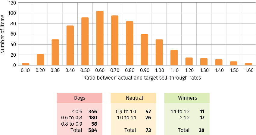
The benefit for a retailer of identifying the dogs and winners in the early season is to make changes for their promotion offer levels that fit the sell-through rate. Consider a retailer that runs a promotion at the brand-category level (for example, all Tahari women’s sweaters will be priced with the same discount). This retailer can do the above sell-through analysis for each brand-category group early in the season, and take action depending on the number of dogs and winners as follows:

• If only a few sizes and colors are dogs in this group, then a retailer can select those items to go on clearance first, and eliminate the need to go with deeper discounts for the entire promotion offer group.
• If one of the styles is dog, then a retailer can break that style into different promotion offers and price them differently.

5.5 Breakage caused by size variation

Breakage refers to the situation when some item variants (certain sizes, colors, etc.) go out of stock while other variants are still in stock. Breakage can be caused by uneven inventory levels for different variants, uneven demand, or both.

The breakage factor can be forecasted based on the total number of variants, the initial stock levels for each variant, and the total forecasted inventory on hand. For example, if we have a product with 5 variants and the initial inventory is 1 unit per variant (so 5 units in total), then the initial breakage factor is 1.0 (all variants are in stock). Once we sell one item and on hand inventory decreases to 4 units, the breakage factor also decreases to 0.8 (one of 5 units will be out of stock). Once we sell two items and the on hand inventory goes down to 3 items, the breakage factor will be 0.6, and so on. If the initial inventory is more than one unit per variant, the dependency will be more complex. For instance, if we have 5 units per variant (25 units in total), then the breakage factor will stay equal to 1.0 until we sell at least five units, and then will slowly decrease. Once the 5th unit is sold, there are only 5 chances out of 125 that some item will go out of stock (i.e. all five units sold will be of the same variant) if the demand for all variants is assumed to be the same. An example of breakage functions is shown in Figure 13. These curves can be computed either analytically or using Monte Carlo simulations for different initial parameters and demand distributions.

Figure 13. Examples of breakage curves for an item with 5 size variants. Each curve corresponds to a certain initial level of inventory (from 1 to 5 units per size variant). The demand for all variants is assumed to be the same. Breakage also depends on the number of possible sizes: one out of stock size matters more for a product that has just 5 sizes compared to a product that has 10 sizes.

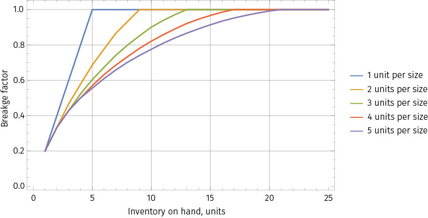
Incorporation of the breakage factors into the seasonal pricing model is very important, especially in a business that is size intensive, like apparel or footwear, as it allows us to differentiate the content of inventory units. The breakage factor is typically incorporated as a demand multiplier.

5.6 Price optimization model for seasonal items

The factors that we discussed above are the main components that a retailer uses to build a pricing model for seasonal items and, as you can tell, is different compared to the pricing model for replenishable items. It does not usually consider cross effects like cannibalization or affinity, since it is very unusual for retailers to price seasonal items individually. Promotion offers usually stays at the rack level, and each rack contains different styles, colors, and sizes. Also, seasonal items are more of a fashion style than the basic style of replenishable items, so the substitution impact is much smaller.
Two unique factors for seasonal model are seasonality and breakage. Seasonality is important because the selling period for seasonal items is much shorter than the basic replenishable items, and the demand for seasonal items changes a lot from one week to the other. With limited inventory on hand, breakage is another important factor to discount your normal demand because you can only sell what you have in stock. All these factors are summarized in Figure 14.

Figure 14. The main factors and effects that need to be accounted for in a pricing model for seasonal items.

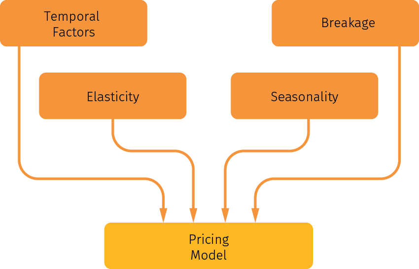
The method to incorporate the above factors into the optimization model is as follows:

1. Develop a baseline demand for the entire selling period by week with no discount prices.
2. Incorporate elasticity to estimate demand with the price change/discount.
3. Multiply that demand by a weekly seasonality factor, holiday factor, and breakage factor.
4. Run what-if modeling for every possible weekly price combination and pick the highest sales revenue option for the entire life of the product, taking inventory constraints into account.
5. Build business rules to guardrail the discount options. For example, the deepest discount allowed before Christmas is 70% off for high-low products, and 50% off for mid-low products. Another example is that an item can only be on sale for 6 weeks out of 9 weeks based on the legal requirement.

Similar to modeling for replenishable items, modeling for seasonal items can take advantage of machine learning methods and train a non-parametric revenue model. This can incorporate econometric parameters like breakage, and learn some parameters like seasonality directly from the sales data.

Another important area where machine learning can be helpful is in the planning of flash sales (short-term sales events). Such events have many common features with seasonal sales (inventory constraints, breakage, etc.), but often go at a much faster pace (weeks or even days). Therefore, online learning and reinforcement learning methods that can estimate price-demand functions based on very few samples are usually beneficial.

6. Conclusions

Compared to the traditional cost plus or value-based pricing methods, sophisticated modeling to optimize prices can help retailers improve their profits substantially. The pricing impact is immediate, and is the most vital component when it comes to making money for the retailers.

A pricing strategy is also the most complex strategy that retailers can execute successfully, since pricing touches everything in the retail operation, and everything touches pricing as well. Despite recent advances in analytics, decision-support tools, and methodologies, retailers are finding that off-the-shelf pricing optimization products are still not enough to keep pace. Not all retailers are the same: they all carry different products and have unique ways of managing their products, so it is very hard to fit a one-size-fits-all kind of pricing modeling. Some large retailers own more than 10 off-the-shelf price optimization products that they use for different product lines, and they still have to spend millions of dollars to customize the tools to make them fit their own needs. A pricing strategy is also the most complex strategy that retailers can execute successfully, since pricing touches everything in the retail operation, and everything touches pricing as well. Despite recent advances in analytics, decision-support tools, and methodologies, retailers are finding that off-the-shelf pricing optimization products are still not enough to keep pace. Not all retailers are the same: they all carry different products and have unique ways of managing their products, so it is very hard to fit a one-size-fits-all kind of pricing modeling. Some large retailers own more than 10 off-the-shelf price optimization products that they use for different product lines, and they still have to spend millions of dollars to customize the tools to make them fit their own needs.

A custom price optimization suite is the key to ensure that retailers stay competitive and successful in this tough environment. In fact, the new digital era stemming from big data, mobile commerce, and the explosion of omnichannel retailing has meaningfully changed the retail environment. In this era, a set of robustic pricing optimization products to make the retailer profitable is not an advantage, but a requirement.