Selecting, training, evaluating, and tuning the model

In previous posts we have discussed the steps needed to understand and prepare the data for Social Movie Reviews. Finally, it is time to run the models and learn how to extract meanings hidden in the data. This blog post deals with the modeling step in the Data Scientist’s Kitchen.

Modeling activities 

At the modeling phase we should select a particular model (or several of them), design the experiment, build the model(s), and assess them. First, however, let’s remind ourselves that our approach is to use as simple a model as possible that can still be effective. Model performance assessment will be based on the corpus of 5,000 manually labeled tweets from Niek Sanders, and visualized with an ROC curve. We will build two models:  Naive Plus/Minus and Logistic regression. The feature extraction process will use the root word dictionary. So...

Naive Plus/Minus model

The simplest model possible is a lexicon-based “Naive Plus/Minus.” For this model a text is shown as a point on a plane. (See below).

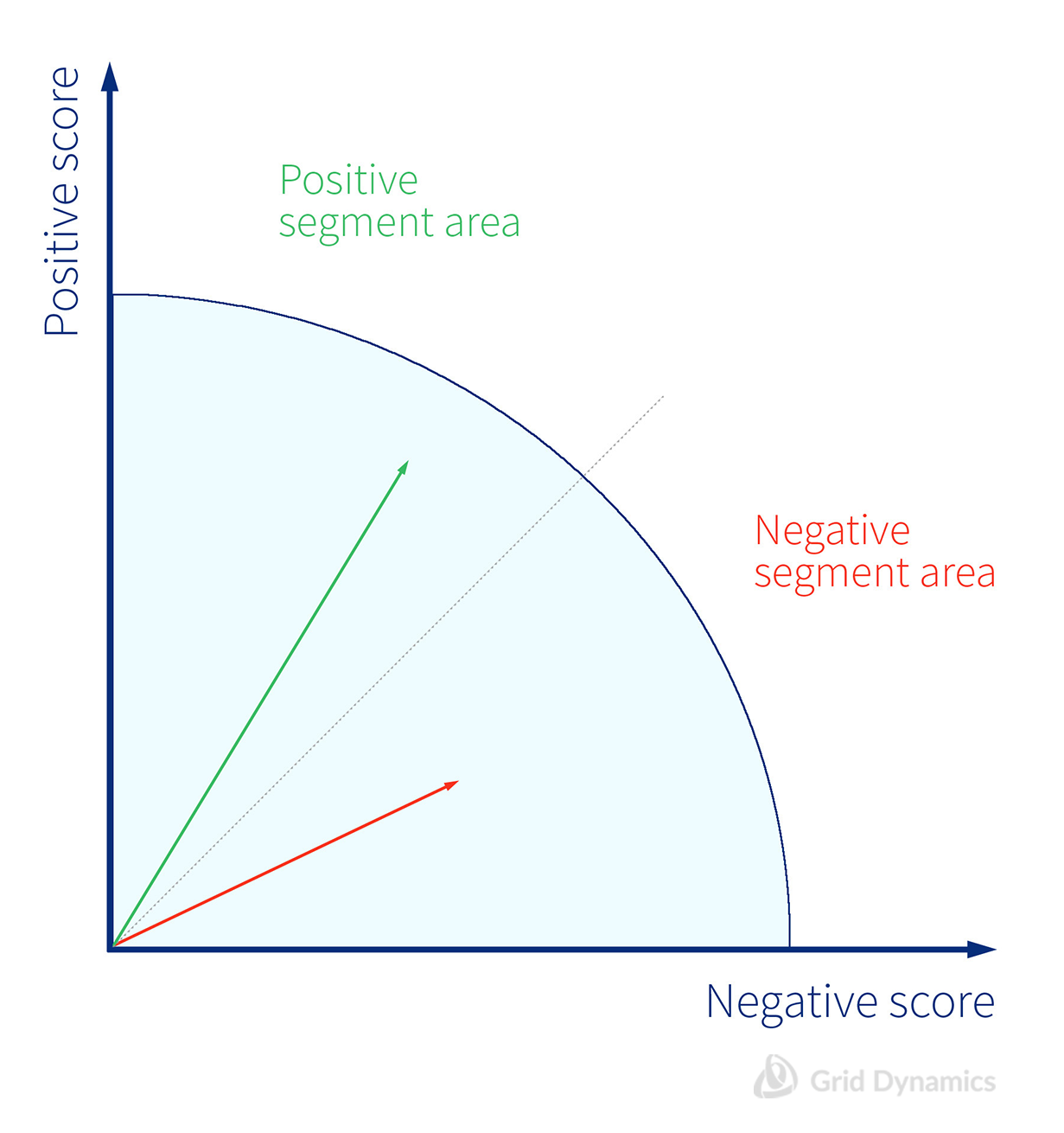
The positive and negative scores are two coordinates. They are calculated as the sum of individual scores for positive and negative words matched to dictionary entries. If the point is above the dotted line the overall text is considered positive. Otherwise, it’s considered as containing a negative sentiment. (See the red arrow.) The separating-line (the dotted one) may have different incline angle resulting in different classification results. This approach is based on the “naive” assumption that an entire text sentiment may be concluded from individual words in the tweet bearing negative and positive emotional loads. That’s why the approach is called “Naive Plus/Minus.” Continuing with our example from the “Data preparation” section in Post #5 in this series, we have a tweet transformed in a set of words from the dictionary.

Now we need to transform it into a vector of scores for every word taken from the dictionary.

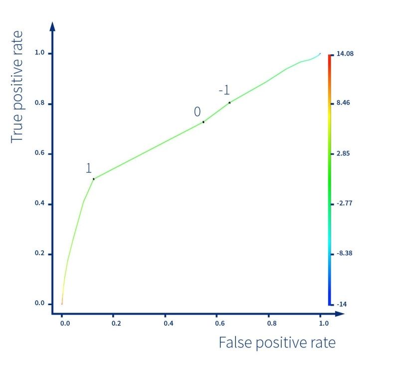
The simplest way to understand where the point with coordinates (1Neg, 5Pos) is to sum the coordinates. In our case the final score for the tweet “Doctor Strange is truly an amazing piece of movie.. fighting the devil.. cool stuff.” is 4. The zero threshold corresponds to the 450 separating line. Given that the threshold is 0, we classify the tweet as positive. For another threshold, say 5, classification would be the opposite. We ran our test dataset, 5K manually labeled tweets from Niek Sanders, through the classifier. On the diagram below an ROC curve is shown for the Naive Plus/Minus model with the changing threshold

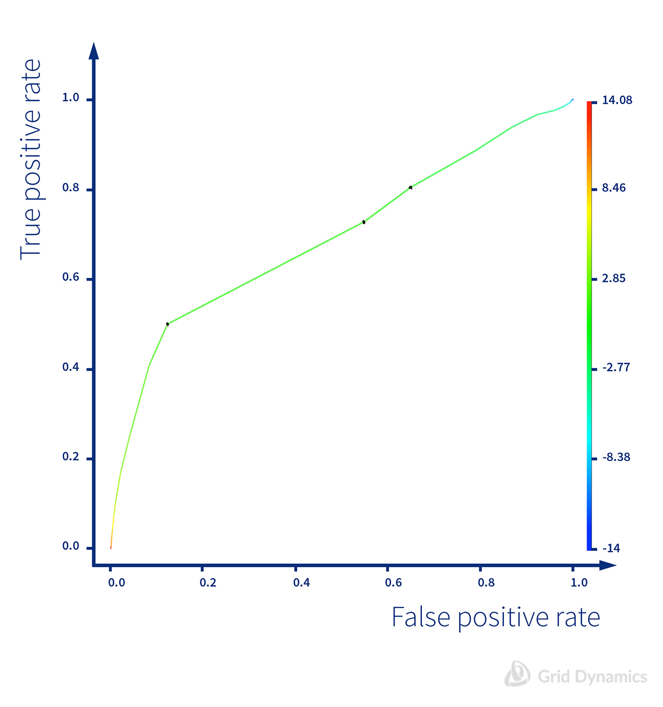
On the curve you can notice numbers: 1 (the most left), 0 and -1. It positions of corresponding threshold values. The colorful scale on the right shows distribution of the threshold values across the curve.

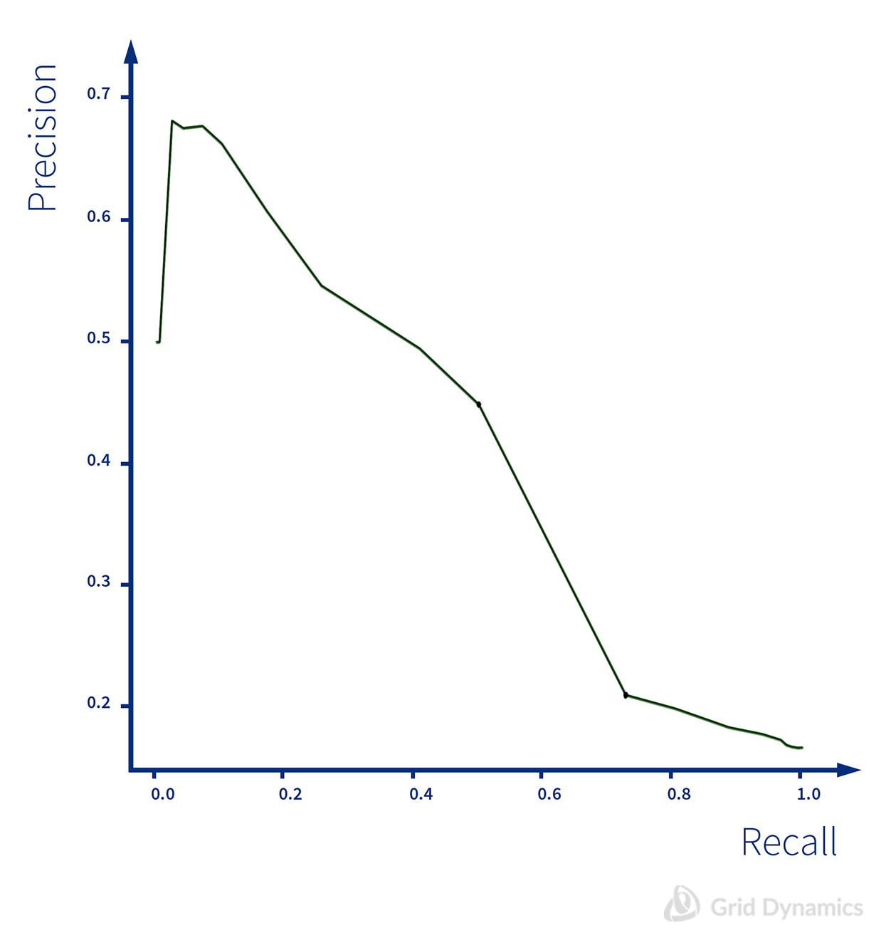
Another diagram showing the model performance is precision vs. recall:

Logistic regression model

Logistic regression is a binary statistical model used to predict a probability of one event based on several independent observable variables. The idea behind this is that there is a logistic curve that looks pretty much like continuous probability distribution.

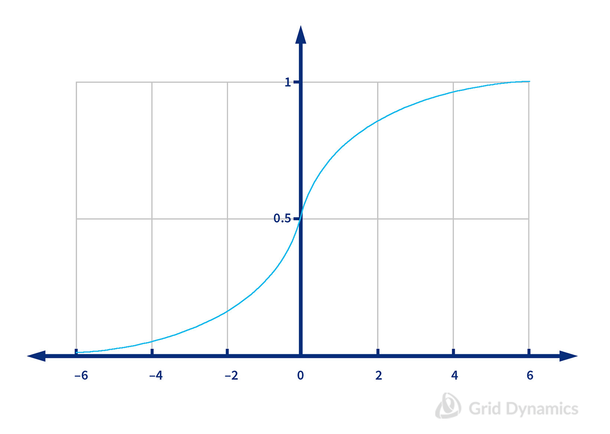
The logistic function formula is 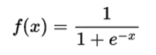 . In order to use the model to predict negative tweets, we should transform the tweet into a number so that a negative tweet would reflect a big positive value on the graph (so the predicted probability of it “being a negative” event would be close to 1), while a positive tweet would reflect in a big negative value (predicted probability of “being a negative” event would be close to 0). 

Although we could use all words that we have in our training dataset, that would give us a very high dimensional task. To deal with it, we would need to reduce dimensionality by identifying and excluding unrelated words like prepositions, pronouns, articles, sentiment-neutral nouns, verbs, and adjectives. This is the work of building a dictionary. So to maintain focus on our main goal, we decided to reuse an existing dictionary, the one with root words.

To go with Logistic Regression we should transform our tweet into a vector of binary variables reflecting presence/absence of every word from the dictionary in the tweet. A short sample of the full vector is shown below:

Having transformed all texts from the training dataset, we get the binary matrix and can train the model. The training will result in a set of coefficients corresponding to every word from the dictionary. The final training dataset consists of 25000 vectors of 1268 words. In turn the test dataset, 5K manually labeled tweets from Niek Sanders, is run through the logistic model.

Evaluation

To decide which model performs better, and what to do next, let’s first have a look at the ROC curve and Precision vs Recall diagrams for both models.

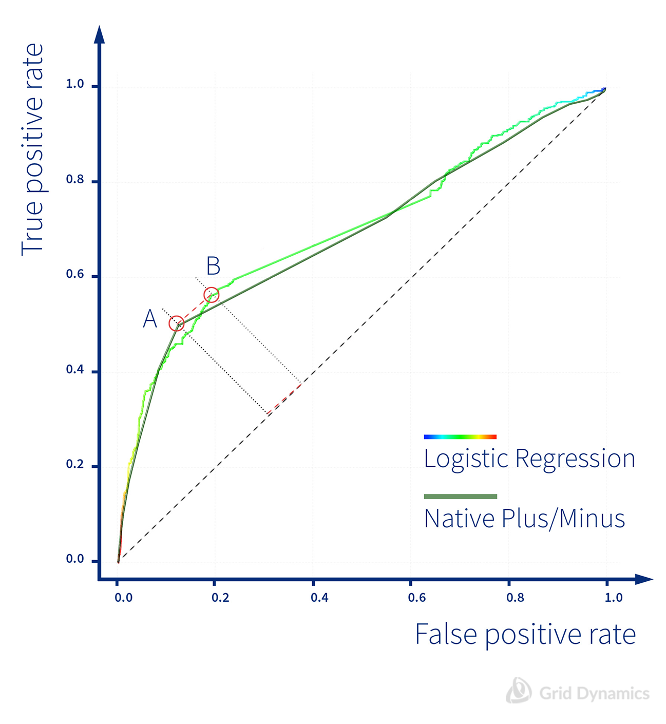
Does point A or B correspond to better performance? To read the above diagram properly and to understand the meaning of a  0.1 change in TPR or FPR, we need to recall that the test dataset has skewed classes. There are 572 negative and 2852 positive samples. So an increase of 0.1 in TPR means 57 more correctly identified negative tweets while an increase of 0.1 in FPR means 285 misclassified positive tweets. The difference between points A and B is equal to random guessing -- that is clearly confirmed by the A-B line, which is almost perfectly parallel to the diagonal line. That means the Naive Plus/Minus model demonstrated better performance than Logistic regression. And there is another angle to evaluate the model quality, the Precision vs Recall curve:

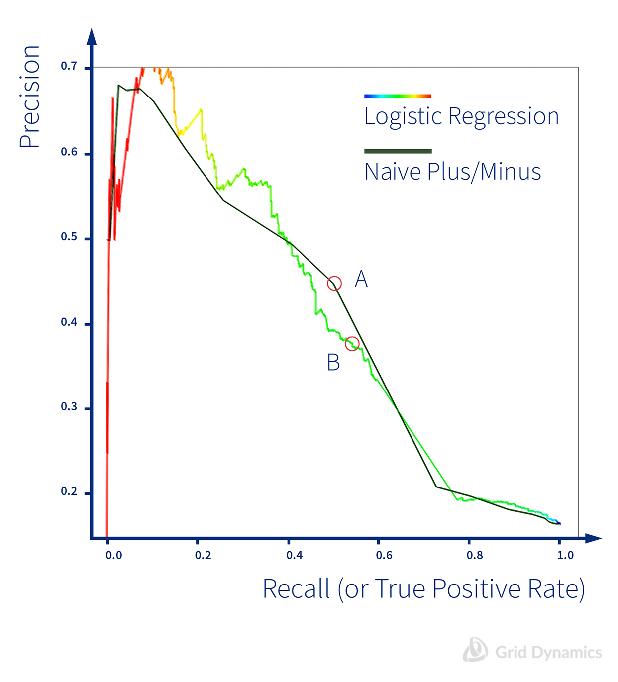
The scale for both axes is equal on this diagram. Here we can clearly see that the Logistic regression outperforms Naive Plus/Minus in some areas, however this area corresponds to a pretty low Recall level --less than 40%. Points A and B on the diagram correspond to the respective points on the ROC diagram. So, the Precision vs Recall diagram clearly confirms that point A corresponds to the better model. In terms of correctly classified negative and misclassified positive tweets, it looks like in the confusion matrix below.

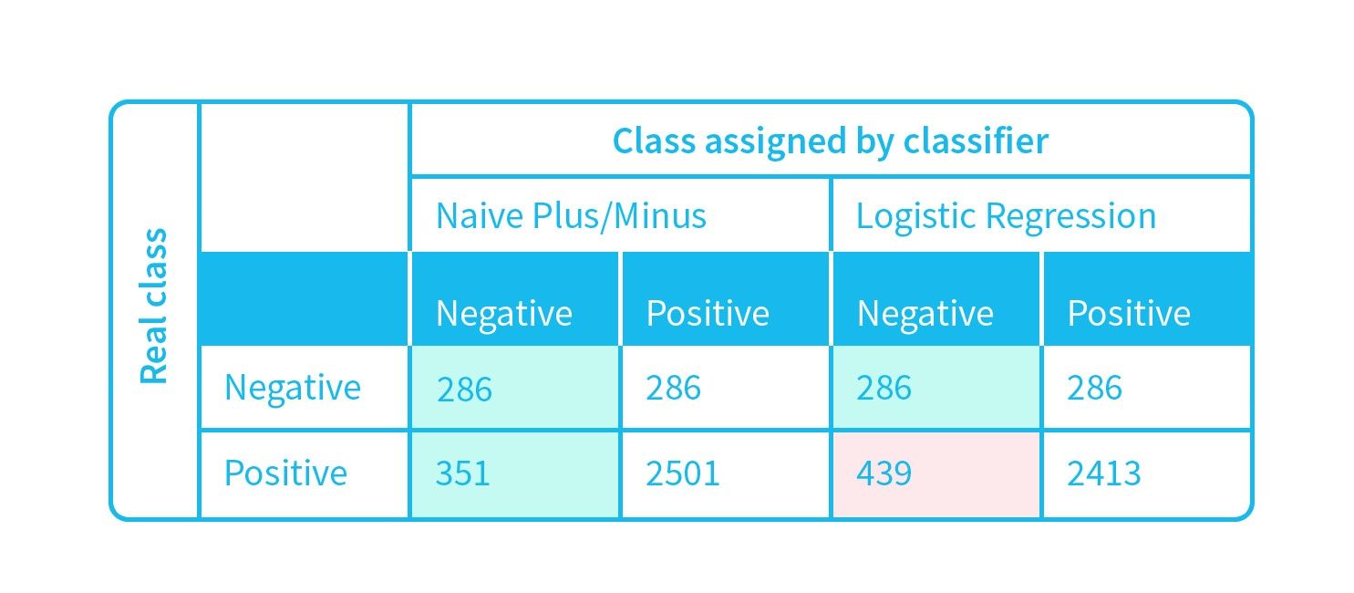
So our research for a sentiment analysis model ended up with rather surprising result: the ultra-simple Naive Plus/Minus model outperforms the more comprehensive Logistic regression model while using the same dictionary. That means the coefficients in the dictionary created by Finn Arup Nielsen are more efficient comparing to “weights” or “estimates” by the Machine Learning algorithm based on positive and negative movie reviews -- in our case from IMDB. This is surprising, as the dictionary author states in the paper,“A new ANEW: Evaluation of a word list for sentiment analysis in microblogs,” that the words were scored manually based on a subjective perception.

Is there a room for improvement in the model? Definitely. Please recall that we heavily simplified the feature extraction process. This is definitely the first place for improvement. We could address synonym challenges, semantic smoothing, typo correction, and many other aspects of our samples. We could build our own dictionary. Do you remember that we mentioned three dictionaries in the beginning? But in the end we are speaking about just one. Why? Of course, we are curious, so we quickly tried Jeffrey Breen’s unigram dictionary. Both models performed much worse with this dictionary. See for yourself; check the ROC curve for logistic regression with both dictionaries.

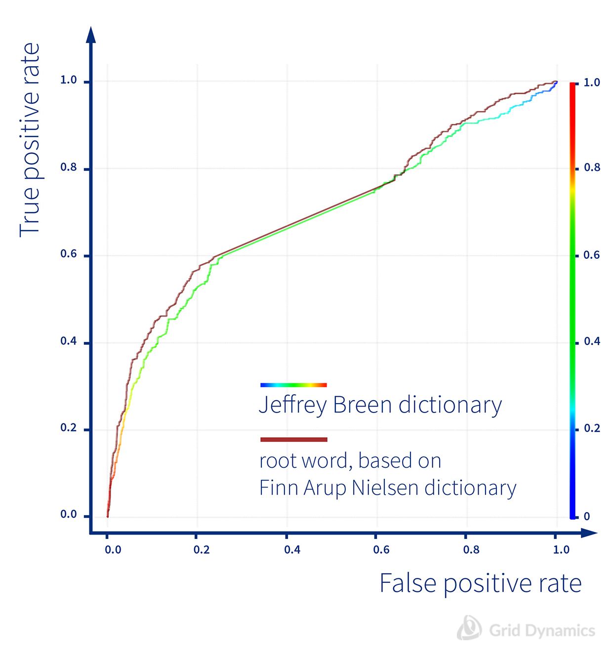
As you can see, the dictionary with 4K words didn’t bring any value comparing to 1.5K dictionary. That might mean the performance of our model is rather limited with the training dataset we used. It pretty well corresponds with the fact that the manually-scored dictionary works better. So one additional way to improve the model’s performance is finding a better training set, e.g. by employing the Amazon Mechanical Turk (AMT) project, as was mentioned by Finn Arup. On the way of feature extraction we also could try to extract more information from the text e.g. perform part-of-speech tagging as this data is used in MPQA Subjectivity Lexicon. Another dimension for possible improvements is trying very different models, for example, nonparametric regression like Random Forest or create other ensembles based on models we have already built. Also we could try non linear models like Deep Learning with neural networks.

We now have a model that can classify tweets as positive or negative, so we have everything we need to perform further analysis and visualise our insights. In our next post we’ll talk about how to do that.