


As the world undergoes the digital transformations, accelerated by the global pandemics, omnichannel shopping experience becomes a new norm. Ship from Store turns out to be an important step on the path of establishing effective and convenient retail practice.
But the transformation brings its' own challenges and demands for new ways of business practices and business optimizations. Large retailers that operate hundreds of stores now face a question on how to choose the best way of fulfillment that is both cost effective and convenient. Traditionally, Order Management Systems (OMS) choose the optimal route for each order independently which often leads to sub-optimal results. In this article we want to present an alternative approach, leveraged by one of the largest US department stores, where we looked for an optimal fulfillment considering all in-flight orders over a time window.
By doing so, they were able to achieve 50% less order splits, double-digit EBIT improvement for optimized orders and multi-million annual savings.
Order cool down period
Important fact that makes this approach feasible is that typically eCommerce sites have certain cool down period while customers are allowed to make changes to their orders before those are pushed down to fulfillment. This allows to accumulate a larger number of orders for simultaneous optimization, without a need for immediate processing.
Example
Let's take a look at a small example. Assume that we have three incoming orders, the same item in each, but with different shipping destination. And those items are available in few stores, with different costs associated with each store and destination combination.
| store A | store B | store C | |
|---|---|---|---|
| customer 1 | 2 | 5 | 6 |
| customer 2 | 7 | 19 | 20 |
| customer 3 | 8 | 15 | 18 |
If we would follow "per order" optimization (in red), then the first customer order would be shipped from store A, 2nd - B and third - C; with a total cost of 2 + 19 + 18 = 39.
But if we try to optimize all three orders together, we can see a better option 1 - C, 2 - A, 3 - B (marked in green), that has cost of 7 + 15 + 6 = 28.
In this example we can see that leveraging global optimization allowed to introduce some savings, but when we multiply it over thousands of orders this might make a noticeable increase in business efficiency. Let's talk about how we can implement that.
Cost
While mathematical approach requires us to present a cost of shipping as a single number, it does not have to be an exact monetary cost of shipment, but can be a derived score that combines many business incentives associated with the shipment:
- The actual shipping cost C 𝑖,𝑗, which ultimately can be a non-linear function depending on total weight of items in shipment and distance,
- Projected time on the shelf in the store, 𝑃𝑖,𝑗
- Promised delivery time 𝐸𝑖,𝑗
- Count weeks before the item expires or becomes obsolete
- Number of total shipments in order
And a certain weight can be associated with importance of each goal, so for example it could look like:
𝐶𝑜𝑠𝑡 𝑖,𝑗 = C 𝑖,𝑗∗𝑊𝑐+𝑃𝑖,𝑗∗𝑊𝑝+𝑆(𝐸𝑖,𝑗)∗𝑊𝑒, where S(x) is a sigmoid function
Brute Force Combinability
Naive approach could be to just try every possible combination and choose one with the least cost. Unfortunately but predictably that becomes quite expensive as soon as number of orders grow. With the example below (3 orders and 3 stores), we only had to compare 27 combinations, but let's take a look how this number grows.
| 3 customers | 4 customers | 5 customers | 6 customers | 7 customers | 8 customers | 9 customers | 10 customers | |
|---|---|---|---|---|---|---|---|---|
| 2 stores | 8 | 16 | 32 | 64 | 128 | 256 | 512 | 1024 |
| 3 stores | 27 | 81 | 243 | 729 | 2187 | 6561 | 19683 | 59049 |
| 4 stores | 64 | 256 | 1024 | 4096 | 16384 | 65536 | 262144 | 1048576 |
| 5 stores | 125 | 625 | 3125 | 15625 | 78125 | 390625 | 1953125 | 9765625 |
| 6 stores | 216 | 1296 | 7776 | 46656 | 279936 | 1679616 | 10077696 | 60466176 |
| 7 stores | 343 | 2401 | 16807 | 117649 | 823543 | 5764801 | 40353607 | 282475249 |
| 8 stores | 512 | 4096 | 32768 | 262144 | 2097152 | 16777216 | 134217728 | 1073741824 |
| 9 stores | 729 | 6561 | 59049 | 531441 | 4782969 | 43046721 | 387420489 | 3486784401 |
| 10 stores | 1000 | 10000 | 100000 | 1000000 | 10000000 | 100000000 | 1000000000 | 10000000000 |
Even if we could check 1 million combinations in a second, it would take almost 3 hours to check all solutions for 10 stores and 10 customers. For 10 stores and 20 customers, it could need more than 3 million years with this approach.
| If we were lucky as species we could probably calculate 14 orders fulfilling in 50 stores before the Sun burns out. |  |
MILP optimization
Luckily there are some optimizations we can leverage. Let's try Mixed-Integer Linear Programming (MILP); this approach appeared in the middle of 20th century, and found it's place in theoretical and practical computer science.
This solution applies to problems when we need to find optimal distribution and minimize some loss, but the distribution parameters can take only allowed values, like we can't ship half of item from store A and another half from store B. Mathematically it is known to be a NP-complete problem; and the specific algorithm we will utilize is called branch-and-cut, you can find some more details below; essentially the idea behind it is that if we know that particular branch of combinations is known to be worse than current best we can skip it entirely.
If we take a look back at our example:
| store A | store B | store C | |
|---|---|---|---|
| customer 1 | 2 | 5 | 6 |
| customer 2 | 7 | 19 | 20 |
| customer 3 | 8 | 15 | 18 |
And assume we have already found across solution 1-C, 2-A, 3-B with cost of 29, we can skip checking any combinations with 2-B, 3-C and 2-C, 3-B, as we know that they can't be better than one we already have.
Deep dive into Branch-and-cut
To illustrate the algorithm better, let's start with introducing some terms.
In the simplest case which we are considering here, we describe each of our possible decisions with variables. Since we can't make everyone happy at once due to our own limitations (physics, budget, facilities capacity, etc.) we imply constraints on our variables. We need them to ensure that solution we find can be actually implemented in real world. Last piece is the target function: it's our formal rule by which we decide what decision is the best (or best we can find).
Each variable can be continuous or integer: for example, if we want to decide how much money we would like to spend on buying stock A and/or stock B, and whether we should buy company C entirely. In this case, we'll have three variables in our model: one continuous variable for investment in A, one continuous variable for investment in B, and one interger (even binary) variable for buying company C. Our constraint will be the total budget: sum of those purchases should not exceed our budget. And our target function can be to maximize expected income given that we know how much money we'll get from each dollar invested in A, B or C.
Note that constraints and target function must be linear with respect to the variables. That means, we can't multiply variables between themselves: we can only add one variable to another, possibly multiplied by some fixed value. This may sound as a big limitation, but it's not: a formal mathematical proof exists that you can formulate any computable problem in terms of MILP and some of it's variations.
Let's write down our shipment problem as MILP:
$d_{ik}$ - amount of items $k$ in client's order $i$
$s_{jk}$ - available amount of items $k$ in store $j$
$c_{ij}$ - delivery costs to client $i$ from store $j$
Vars
$x_{ijk}$ - amount of items $k$ that will be shipped from store $j$ to client $i$
$u_{ij}$ - equals to 1 if we ship anything from store $j$ to client $i$
Constraints
$\sum_j x_{ijk} = d_{ik}$ - order must be satisfied
$\sum_i x_{ijk} \leq s_{jk}$ - we must not exceed inventory
$\sum_k x_{ijk} \leq T u_{ij}$ - set $u_{ij}$ to one if anything is shipped from store $j$ to client $i$ (T - technical big constant: since sum of $x_{ijk}$ can be arbitrary number between zero and $K * max(d_{ik})$, and $u_{ij}$ can take only 0 or 1 values, big constant multiplication is required to ensure inequality works; it's a good idea to keep this constant as small as possible)
Target
$\min \sum c_{ij} u_{ij}$ - minimize total shipment costs
Let's take a look at our earlier example.
In terms of branch-and-cut, all solutions where Store A -> Customer 1 called branch. Value 33$ is called lower bound, because it provides estimate on any possible solution when Customer 1 is served from Store A.
Let's also consider an alternative: we won't ship to Customer 1 from Store A. Well then, we'll try to ship it from Store B. If we also ship Store A -> Customer 2 and Store C -> Customer 3, whole solution would cost us 5$ + 7$ + 18$ = 30$.
Note that this solution is cheaper than lower bound from branch Store A -> Customer 1. That effectively means that we can discard entire branch Store A -> Customer 1: we already found solution in another branch which is better than lower bound in former branch. Such solutions also called upper bound.
LP-relaxation
Another optimization is that instead of actually testing each combination, once some of the variables are bound, we could apply simpler decimal solvers to find best decimal solution for unbound variables and compare it with the known lower boundary. If we find that the decimal solution has better cost, then we would need to test closest integer values and check if they still stand. But if we know that even decimal solution is not better, we can skip that branch altogether.
Using Solvers
There's a number of available MILP solvers both free and commercial. Let's take a look how we can use free CBC solver that is available in the pywraplp module of Google OR-TOOLS package.
First let's load the library and initialize the solver. We also limit max calculation time to 5 minutes. For such problems, it is possible that checking all combinations might actually take years even with the solver, so we need to put some reasonable limit to get 'good enough' estimate.
problem_type = pywraplp.Solver.CBC_MIXED_INTEGER_PROGRAMMING
solver = pywraplp.Solver('Ship From Store: optimal fulfillment', problem_type)
solver.SetTimeLimit(5 * 60 * 1000)
Now, let's define contraints and target for optimization:
X = {}
for i in range(order_count):
    for j in range(store_count):
        for k in range(catalog_count):
            X[i, j, k] = s.IntVar(0, int(orders[i, k]), 'x_{}_{}_{}'.format(i, j, k))

# Create u_ij variables
U = {}
for i in range(order_count):
    for j in range(store_count):
        U[i, j] = s.IntVar(0, 1, 'u_{}_{}'.format(i, j))

# Add constraint: order must be satisfied
for i in range(order_count):
    for k in range(catalog_count):
        s.Add(s.Sum(X[i, j, k] for j in range(store_count)) == orders[i, k])

# Add constraint: do not ship more SKUs from store than available inventory in this store
for j in range(store_count):
    for k in range(catalog_count):
        s.Add(s.Sum(X[i, j, k] for i in range(order_count)) <= availability[j, k])

# Big const
T = catalog_count * np.max(orders)

# Add constraint: set u_ij to one if anything is shipped from store j to client i
for i in range(order_count):
    for j in range(store_count):
        s.Add(s.Sum(X[i, j, k] for k in range(catalog_count)) <= T * U[i, j])

# Set target function
s.Minimize(s.Sum(cost[i, j] * U[i, j] for i in range(order_count) for j in range(store_count)))
Finally, let's run the solver and print the results
res = s.Solve()

sol = {}
# Extract the solution from solver
for k, x in X.items():
    if SolVal(x) > 0:
        sol[k] = SolVal(x)

s.Iterations(), s.Objective().Value(), res, sol
See full code example
def solve_problem_cbc(order_count, store_count, catalog_count, orders, availability, cost):
    problem_desc = 'SFS simple model'

    # pywraplp supports several optimizers, proprietary and open-source
    # We should specify which solver are we going to use
    problem_type = pywraplp.Solver.CBC_MIXED_INTEGER_PROGRAMMING

    # Initializing solver
    s = pywraplp.Solver(problem_desc, problem_type)

    # Create x_ijk variables from model description above
    X = {}
    for i in range(order_count):
        for j in range(store_count):
            for k in range(catalog_count):
                X[i, j, k] = s.IntVar(0, int(orders[i, k]), 'x_{}_{}_{}'.format(i, j, k))

    # Create u_ij variables
    U = {}
    for i in range(order_count):
        for j in range(store_count):
            U[i, j] = s.IntVar(0, 1, 'u_{}_{}'.format(i, j))

    # Add constraint: order must be satisfied
    for i in range(order_count):
        for k in range(catalog_count):
            s.Add(s.Sum(X[i, j, k] for j in range(store_count)) == orders[i, k])

    # Add constraint: do not ship more SKUs from store than available inventory in this store
    for j in range(store_count):
        for k in range(catalog_count):
            s.Add(s.Sum(X[i, j, k] for i in range(order_count)) <= availability[j, k])

    # Big const
    T = catalog_count * np.max(orders)

    # Add constraint: set u_ij to one if anything is shipped from store j to client i
    for i in range(order_count):
        for j in range(store_count):
            s.Add(s.Sum(X[i, j, k] for k in range(catalog_count)) <= T * U[i, j])

    # Set target function
    s.Minimize(s.Sum(cost[i, j] * U[i, j] for i in range(order_count) for j in range(store_count)))

    # For such kind of problems it's a common situation that solution may take years, even with solvers
    # So it's a good idea to set a time limit for solution: when the time runs out
    # the best found solution returned, without any guarantees that it's a best one existing.
    # If time runs out, it's also possible to obtain best found estimate for the optimal solution
    # Here we set time limit to 300 seconds
    s.SetTimeLimit(300000)

    # Solve the problem. "res" variable contains return code for the solution. Description of codes
    # can be found here
    # https://google.github.io/or-tools/java/enumcom_1_1google_1_1ortools_1_1linearsolver_1_1MPSolver_1_1ResultStatus.html
    res = s.Solve()

    sol = {}
    # Extract the solution from solver
    for k, x in X.items():
        if SolVal(x) > 0:
            sol[k] = SolVal(x)

    return s.Iterations(), s.Objective().Value(), res, sol
Execution time
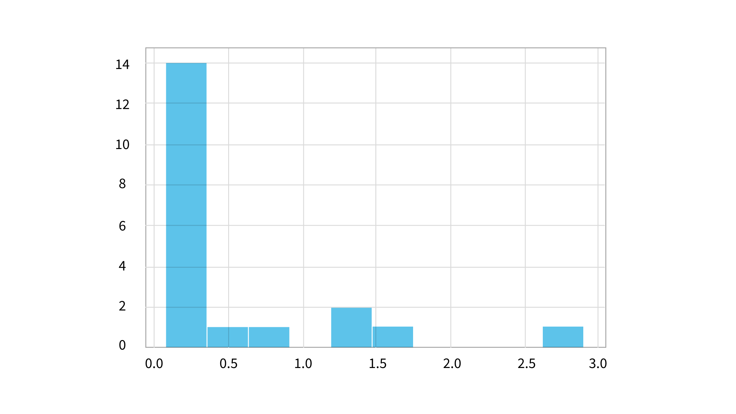
Now let's see how much time does it take. First let's start with 20 orders, 5 stores and 10 items, and do a multiple random runs. All of samples are calculated under 3 seconds, with mean execution time about 0.5 seconds.
But if we double the size and try allocating 40 orders, 10 stores and 20 items, solver can't complete full search in 5 minutes anymore.
Commercial Solvers
So the next step is to see what commercial solvers can achieve. For MILPs, the best two options are Gurobi and Ibm's CPLEX. Here's some summary of Gurobi execution.
Now the execution time distribution for second problem looks much better, with mean execution time under 50 seconds and 90% completing under 90 seconds:
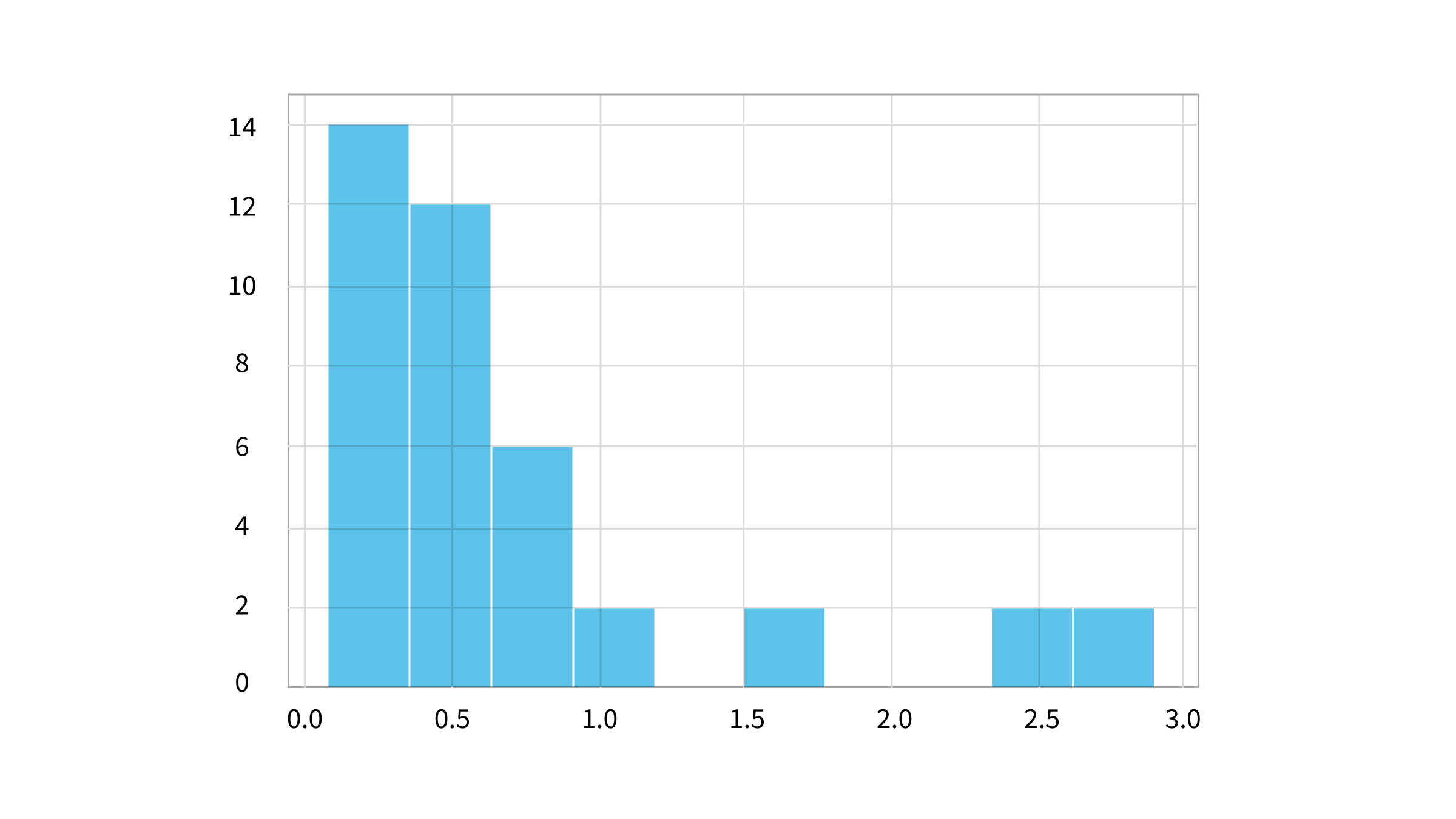
Also the worst case is still solved under 155 seconds, less than three minutes.
Gurobi solver example code
import gurobipy as gp
from gurobipy import GRB

def solve_problem_grb_core(model, order_count, store_count, sku_count, orders, availability, cost):
    # Create x_ijk variables
    x_vars = model.addVars(range(order_count), range(store_count), range(sku_count),
                       vtype=GRB.BINARY,
                       name="x_assign")

    # Create u_ij variables
    u_vars = model.addVars(range(order_count), range(store_count),
                       vtype=GRB.BINARY,
                       name="u_assign")

    # Tell the optimizer that we're looking for minimum-cost solution
    model.modelSense = GRB.MINIMIZE

    # Add constraint: order must be satisfied
    for i in range(order_count):
        for k in range(sku_count):
            model.addConstr(sum(x_vars[i, j, k] for j in range(store_count)) == orders[i][k])

    # Add constraint: do not ship more SKUs from store than available inventory in this store
    for j in range(store_count):
        for k in range(sku_count):
            model.addConstr(sum(x_vars[i, j, k] for i in range(order_count)) <= availability[j][k])

    # Big const
    T = sku_count * np.max(orders)

    # Add constraint: set u_ij to one if anything is shipped from store j to client i
    for i in range(order_count):
        for j in range(store_count):
            model.addConstr(sum(x_vars[i, j, k] for k in range(sku_count)) <= T * u_vars[i, j])

    # Set formula for the target function
    model.setObjective(sum(cost[i][j] * u_vars[i, j] for i in range(order_count) for j in range(store_count)))

    # Run optimization
    model.optimize()

    # Return optimization status code
    # Reference can be found here
    # https://www.gurobi.com/documentation/9.1/refman/optimization_status_codes.html
    return model.Status, model.Runtime

def solve_problem_grb(param_I, param_J, param_K, mat_D, mat_S, mat_C):
    model = gp.Model("sfs")
    return solve_problem_grb_core(model, param_I, param_J, param_K, mat_D, mat_S, mat_C)
How can we improve it further?
The performance of the solver heavily depends on how accurate lower and upper bounds are estimated, and also on the order of branch evaluation: the sooner solver comes across a solution close to optimal, the more effective cutting it is able to leverage, the less combinations it has to evaluate, hence getting optimal solution faster.
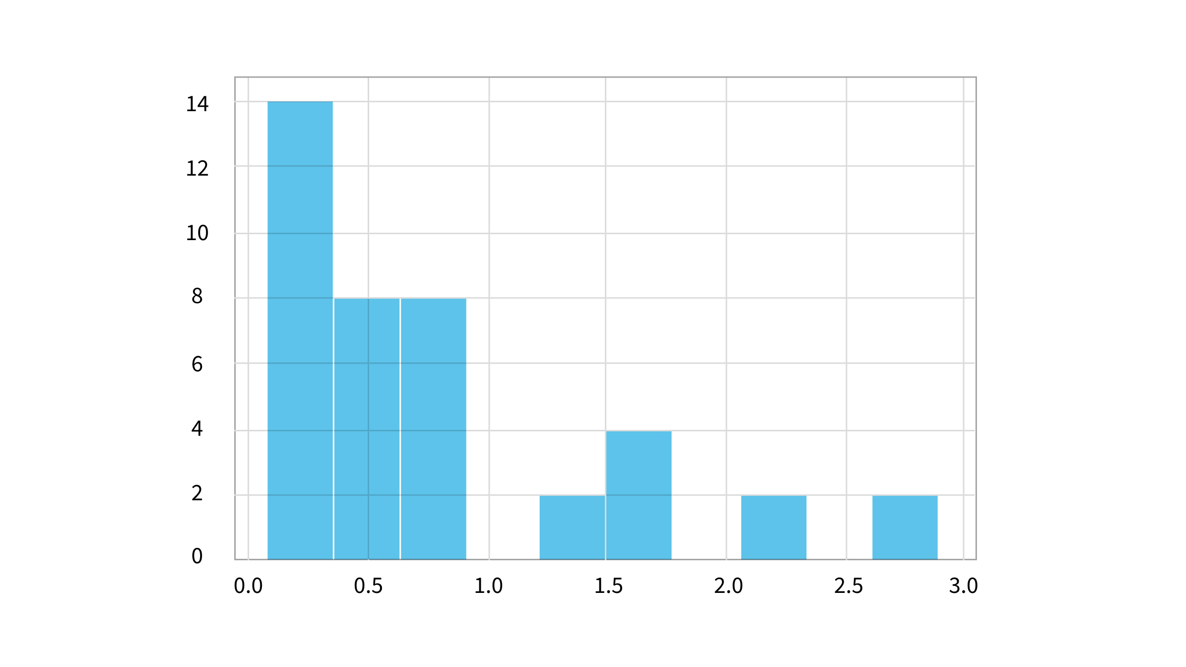
To direct that process solvers use heuristics, where they spend some time evaluating data in order to find most promising order of evaluation, some of it before all calculations, some along the way. By default Gurobi allocates 5% of time to heuristics, but if we override and increase it to 10% we can see much better performance.
m = gp.Model("sfs")

# Default value of m.Params.Heuristics is 0.05
m.Params.Heuristics = 0.1
Now average execution time increased by 1.5 seconds, but 90% decreased by 5 seconds, and the worst case decreased by almost 10 seconds.
Early Stopping
As we can see majority of cases are solved way under the limit, let's see how much less optimal solution for the worst cases we get if we stop early, maybe we don't even need to solve all cases optimally.
So let's try to set max limit to 1 minute, instead of 5. Now we can see that only 20% of cases were terminated due to time out, and the solutions found within the time limit were just 2% to 3% higher than the optimal.
Next Optimization Steps
We need to mention that further accuracy improvement can be achieved with custom lower boundary calculation procedure, but will keep details out of scope of this article. The same applies to heuristic determination: with custom logic based on the domain specifics it's possible to speed up the solver few times.
Conclusion
We have demonstrated how using MILP techniques we were able to introduce cross order optimization into ecommerce ship-from-store order fulfillment. Free and commercial software is available with ready to use solutions, and tuning of those allows to achieve significant performance improvements.