
Street-to-Shop: Is the Future of Fashion Visual Search?
Meet Lucy, a nice young lady and enthusiastic fashion shopper. Spring is in the air and Lucy just passed by somebody wearing this truly amazing dress.
She positively needs to get something like this, right now. Easy! Lucy opens her favorite clothing store’s website, taps the search bar and types in… what? How does she describe this outfit? “Long white sleeveless dress”? Well, she just described this and hundreds of similar dresses.
She could be more specific and describe it as “floral-pattern, white and pink, one-shoulder, maxi dress.” This is, of course, exactly right, but still hardly useful in her online shopping quest.
Isn’t it so much easier for Lucy to just point her phone, snap a picture and instantly find this dress along with many similar looking dresses?
This is exactly the job of the Street-to-Shop fashion visual search solution we will describe.

In this blog, we will talk about how to build a deep learning-based computer vision model that powers the fashion visual search system. We will focus on casual street images and will train the model to recognize fashion items in those images.
The challenge of the street images
When designing a visual search system, dealing with studio quality "shop" images is relatively easy. There is no noisy background to deal with, lighting conditions are consistent, the model is posed, and the subject of the search clearly occupies a majority of the image.
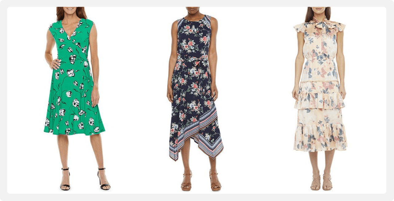
But things get more complicated with real-life smartphone-captured images. There is huge variability in lighting conditions, backgrounds, and in people's poses. Often the search subjects have to be detected among an otherwise crowded image.

High quality visual search systems should be resilient to those variations and should be able to detect and segment apparel images to focus the search on the actual subject.
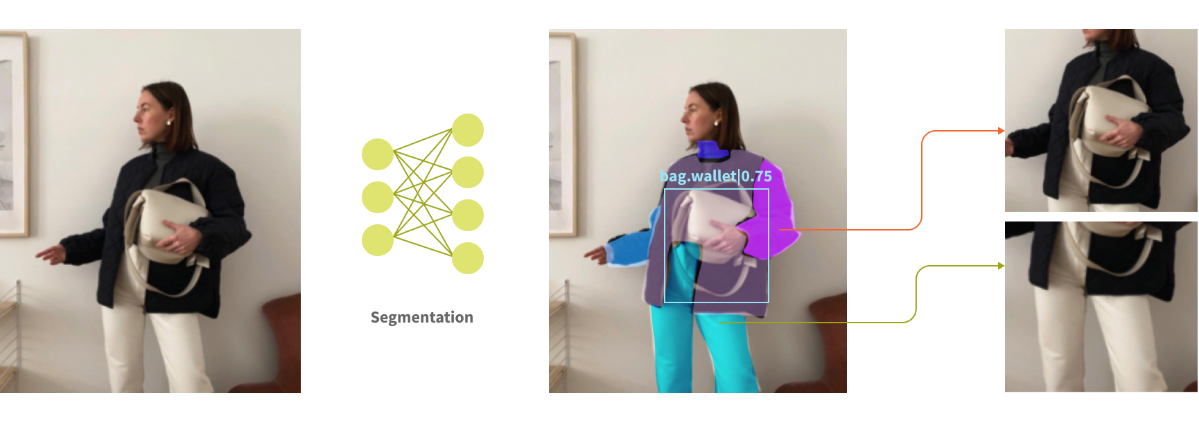
Now, let's review the core of the system - the visual similarity model.
Street-to-Shop fashion search model
Visual search system has two main components: image encoder, which converts user's image into a vector representation and vector index representing all catalog products, encoded by the image encoder.
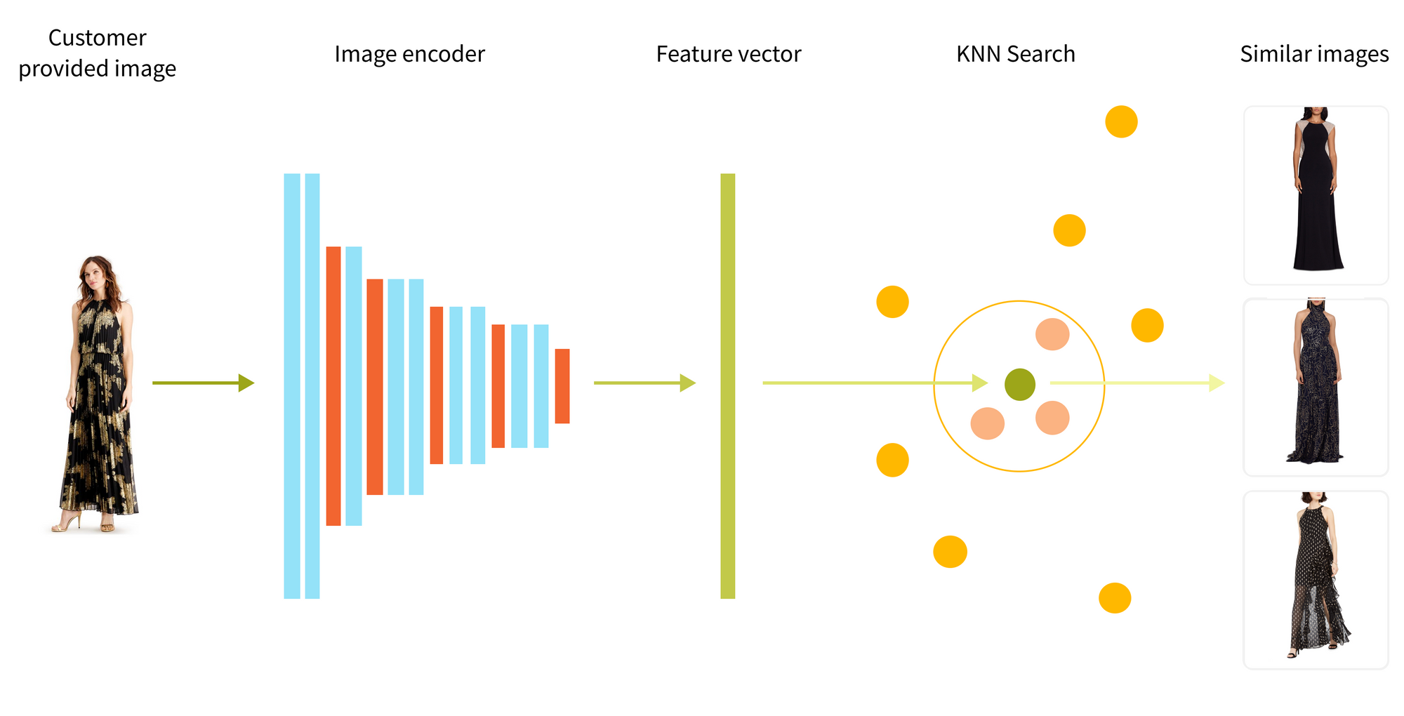
The secret sauce of the visual search is how to train the image encoder to encode items with the similar fashion style in such a way that their vector representation is close to each other according to a vector similarity metric, such as cosine similarity. After that, all we have to do to find similar images is to encode the user's image (let's call it an anchor image) into a feature vector and retrieve K nearest neighboring vectors from the vector index - this will be our search result.
This simple workflow is often enhanced with other components, such as image pre-processing, object detection and segmentation, attribute classification and results post-filtering.
At the heart of the visual search system lies the image encoder powered by a visual similarity model, so we will focus on this component of the system in this post.Image encoder is based on a neural network which consists of an image recognition backbone followed by one or more embedding layers which map the backbone output to the final vector representing the input image. Depending on the application, vector size can vary from 64 to 2048 or even more dimensions.
The image recognition part of the model can be based on convolutional neural network architecture, such as EfficientNet or other emerging architectures such as visual transformers.
Pre-trained neural networks achieve mediocre results in fashion similarity search. We have to re-train and fine-tune our image recognition backbone on apparel data, allowing it to learn the fashion-related features and fashion similarity.
Such retraining requires collecting a large fashion dataset, so let's look into how we built and cleaned our own street-to-shop dataset.
Building Street-to-Shop dataset
In order to teach our visual similarity model to recognize fashion nuances we built a "Street-to-Shop" fashion dataset containing a large variety of apparel images. This dataset maps "shop" items, represented by studio-quality images found in e-commerce catalogs to "street" images, taken by regular people on their smartphones. Each shop product in the dataset should have one or more street images with the same or very similar item. The product and set of similar images is then grouped together into a dataset.
We started with the open source street2shop datasets kindly published by M. Hadi Kiapour et al. It consists of more than 300,000 street and shop images. Unfortunately, this dataset is pretty noisy and requires an extensive cleanup. After cleaning up we obtained only 15,000 shop-street image pairs.
We needed at least an order of magnitude more data to train our models, so we crawled additional fashion images from public sources. The key challenge was to build the shop-street association between images and we used a number of techniques to automate this mining process. We used customer reviews which contained product images, social media tags and a number of other techniques to map shop images to the street counterparts.
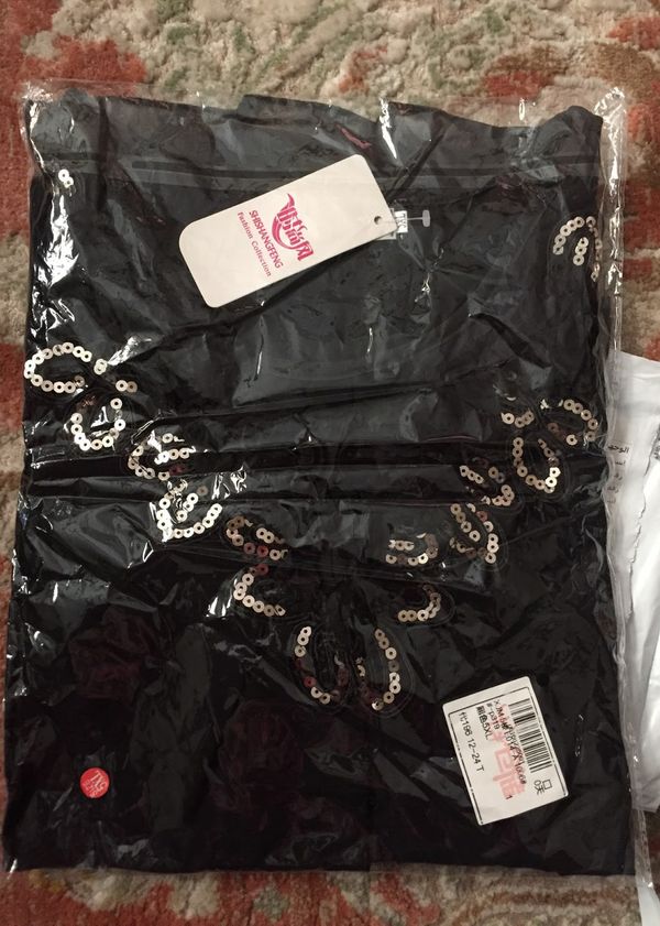
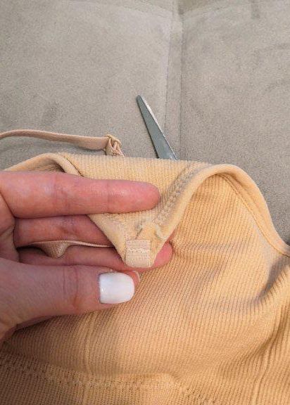
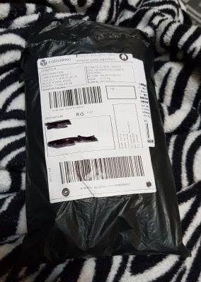
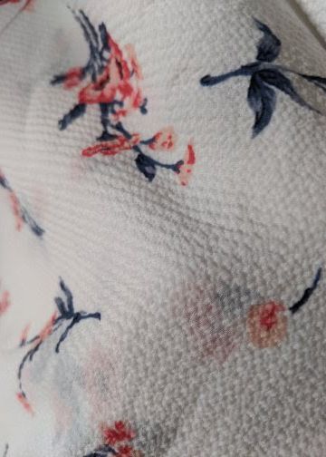
Despite our best efforts, collected data included a lot of noise, such as size tables in the shop images, package photos in the street images, and many other unusable images:
 |
 |
 |
 |
 |
 |
To clean up our Street-to-Shop dataset we used a combination of unsupervised and supervised techniques.
We started from vectorizing images with a pre-trained backbone model, and clustering result vectors with HDBScan and K-means algorithms. We inspected the result clusters and dropped the clusters that contained mostly noise. This eliminated most of the simple noise images like non-apparel pictures and fragments.
For further cleanup we applied a supervised method. We labeled a modest number of images as "noise" and "clean", with equal numbers of samples from each label. Next, we trained a binary classifier on top of a pre-trained backbone. As a result, we got sufficient discriminating power in our classifier and were able to identify and discard the majority of noise images, which represented about 30% of our dataset.
Finally, our dataset contained a lot of near-duplicate images which were not helping the model to train. We eliminated them by performing nonlinear projection of original 768-dimension feature vectors to just 5 dimensions. After calculating pairwise distances we could identify potential duplicates which were too close to each other.
As a result, we obtained about 150,000 usable street-shop pairs across several categories. For example, the dress category contains about 65,000 street-shop pairs.
Model training
To train the visual similarity model we experimented with two main similarity training techniques using Triplet and ArcFace losses. Originally these losses were developed for face and person recognition and re-identification tasks. But it turns out that they work very well for many other similarity search tasks.
Triplet loss
Triplet loss is a classical technique widely used in metrics learning and similarity search. In general training objective looks as follows:
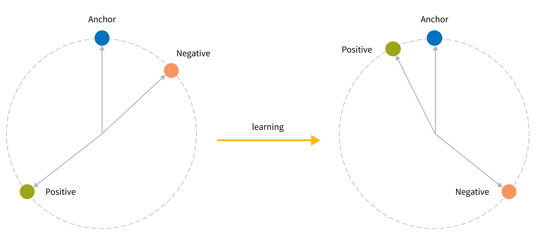
During training we have to send a triplet - 3 images from the same product group into the network and get 3 feature vectors for them. This triplet consists of Anchor - street image, Positive - relevant shop image and Negative - irrelevant shop image. After we calculate feature vectors, we can measure the distance between Anchor and Positive and between Anchor and Negative using a particular vector distance metric, such as cosine distance.
The learning objective is to minimize anchor-positive distance and maximize anchor-negative distance using following formula:

Here, α stands for a margin, by which anchor-negative distance should be bigger than anchor-positive. If anchor-negative distance plus margin is lower than anchor-positive distance, we will produce a gradient and update network weights to push the negative sample further from the anchor and pull the positive sample closer to the anchor.
Triplet loss allows us to rank images by similarity, which is hard to do using classical loss functions used for multi-label classifications.
The biggest challenge in using the triplet loss approach is that it requires negative samples. A good negative sample will be "hard", e.g. it will not be obviously irrelevant, to allow the model to learn the nuances. We need a lot of such samples, so we need to implement a special approach to mine such negatives from data.
A naive approach is just to use a random image from a different product group as a negative sample. There is still a chance that the random image can be very close visually to the product anchor, yet those odds decrease with increasing the number of samples. More complex techniques to collect negatives require user engagement data and we can discuss them in future blog posts.
After we collected negative samples there are several optimization techniques which would help the model learn significantly faster and achieve much better quality. This technique is called "hard" mining. The main idea is to evaluate the batch of samples and find triplets with the largest loss value. Similarly, "semi-hard" mining approach focuses on triplets that have loss values somewhere near the middle of the loss distribution. For more details, we can recommend a Triplet Loss and Online Triplet Mining in TensorFlow . A common pitfall of using "hard" mining in combination with collecting negatives using random sampling. This can backfire, because it is possible that randomly sampled similar images will be boosted on top and confuse the model. In our experience, we found that semi-hard mining brings the best results.
ArcFace
ArcFace is another popular technique for similarity metrics learning which was introduced after a Triplet loss. This technique originally was designed for face recognition as well.
As opposed to triplet loss, we do not need to provide negative samples in the dataset. It is enough to pose a multi-class classification problem where shop images grouped by product represent classes and we classify street images to those classes.
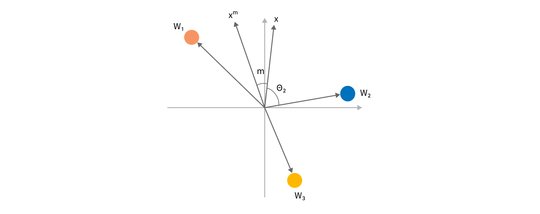
To understand the key idea behind ArcFace loss, let's consider a toy example where we are building an image classifier which has 2 embedding dimensions and 3 classes.

A toy image classifier with two-dimensional embeddings and 3 classes
If we L2-normalize the embedding and weights we can consider each row in a classifier matrix as a vector of length 1. Dot product Wjtx is treated as class j probability. At the same time, we can view this product as a cosinus of the angle between our embedding and a vector Wtj pointing to a "class center". Indeed, if this angle is zero, we will classify x as class j with probability 1. So, we can add a loss to minimize this angle and entice the encoder to point image embedding closer to the direction of the correct "class center". However, it is not enough just to have the embedding to be slightly closer to the ground truth class center than the second-closest class. We want it to be significantly closer to the target. For that purpose, we are adding a constant angular margin m to the angle we are trying to minimize. After adding this margin, we convert our modified angle back to the result of the dot product and send it to the standard softmax layer.
As a result of this optimization, we keep our classes compact and separate, e.g. we minimize angular distances for embeddings belonging to the same class and maximize angular distances between centers of different classes, which significantly improves reliability of classification and the quality of our embeddings.
Here, θ is the angle between embedding and class center, m is a margin we discussed and s stands for scale parameter. Scale parameter changes the shape of the vector space. The higher the scale, the more sensitive product representation becomes to the changes in colors or shapes of the item.
In our experiments, ArcFace loss showed much better results compared with triplet loss with approximately 20% higher scores in MAP@20 metric. Based on this result, we continued our future improvements using ArcFace.
Training protocol
We separated the training process into several phases depending on the training backbone and loss function.
We tried different learning rates and unfreezing policies, and identified the following training protocol to perform best for our case:
- Warm-up phase: training with frozen 5 bottom layers for 1 epoch
- Active training phase: unfreezing layers from 6 to 3 for 10-20 epochs
- Fine-tuning phase: 10x decrease in learning rate and training for 10-20 more epochs.
- Testing result model on the reserved test dataset
In case of Triplet loss, data is grouped by product and in each batch we send an anchor product, at least one positive product for it and at least one negative. In the case of ArcFace we don't need to add special processing for batch content, however before we start training we need to create ground truth with class codes for our anchors.
Train/test/validation split have standard 80/10/10 ratio.
Results Evaluation
Results were evaluated by Mean average precision
We didn't use NDCG metrics as we wanted to concentrate on exact matches and ranking of similar items is secondary to our main objective to find the correct catalog product by its street image. If the high quality ranking of similar styles is a goal, we can employ customer interaction data to train for this objective.
The mean Average Precision is derived from the Average Precision (AP)
In which TP stands for True Positives, whereas N(k) and TP seen can be calculated from the following formulas.
For the perfect case, the AP will be equal to 1, which implies that the model can correctly prioritize all the TP to be in the highest ranks.
So far, we’ve only got an AP@k for a single query. To find MAP@k, all we need to do is to calculate the average.
Evaluation process
When the evaluation phase starts we take validation's anchor images and generate vector index using models from the last training phase. When the index is created, we run KNN search for each anchor vector in the index and compute AP@5 for each top 5 KNN result set. After all results collected we compute MAP@5 using previously collected AP metrics.
We used the top 5 results in our work, but the k parameter should reflect how many results the user will be interacting with. Usually numbers are 1,5, 24 and 36.
The same process happens at the end of training with a test set.
Choosing the model backbone
We tested a number of popular SoTA backbones to choose the best for our case:
- Efficientnet-b3 backbone, pre-trained on imagenet
- Resnext101_32x8d backbone, pre-trained on instagram photos dataset
- Data-Efficient Image Transformer (DeiT) backbone, pre-trained on imagenet
We got the following results for backbones using evaluation and test datasets (results shown for the dresses category only)
| Model backbone | MAP@5, eval | MAP@5, test |
|---|---|---|
| resnet50 | 0.668 | 0.503 |
| resnext101_32x8d | 0.689 | 0.529 |
| resnext101_32x8d_wsl | 0.752 | 0.609 |
| efficientnet-b3 | 0.680 | 0.521 |
| DeiT-base-224 | 0.740 | 0.579 |
WSL pre-trained weights usage is restricted to research by license, so we used the next best candidate: the visual transformer-based DeiT network.
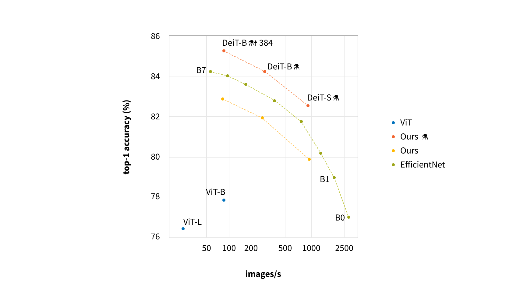
DeiT is a state-of-the-art vision transformer implementation, provided by Facebook research.
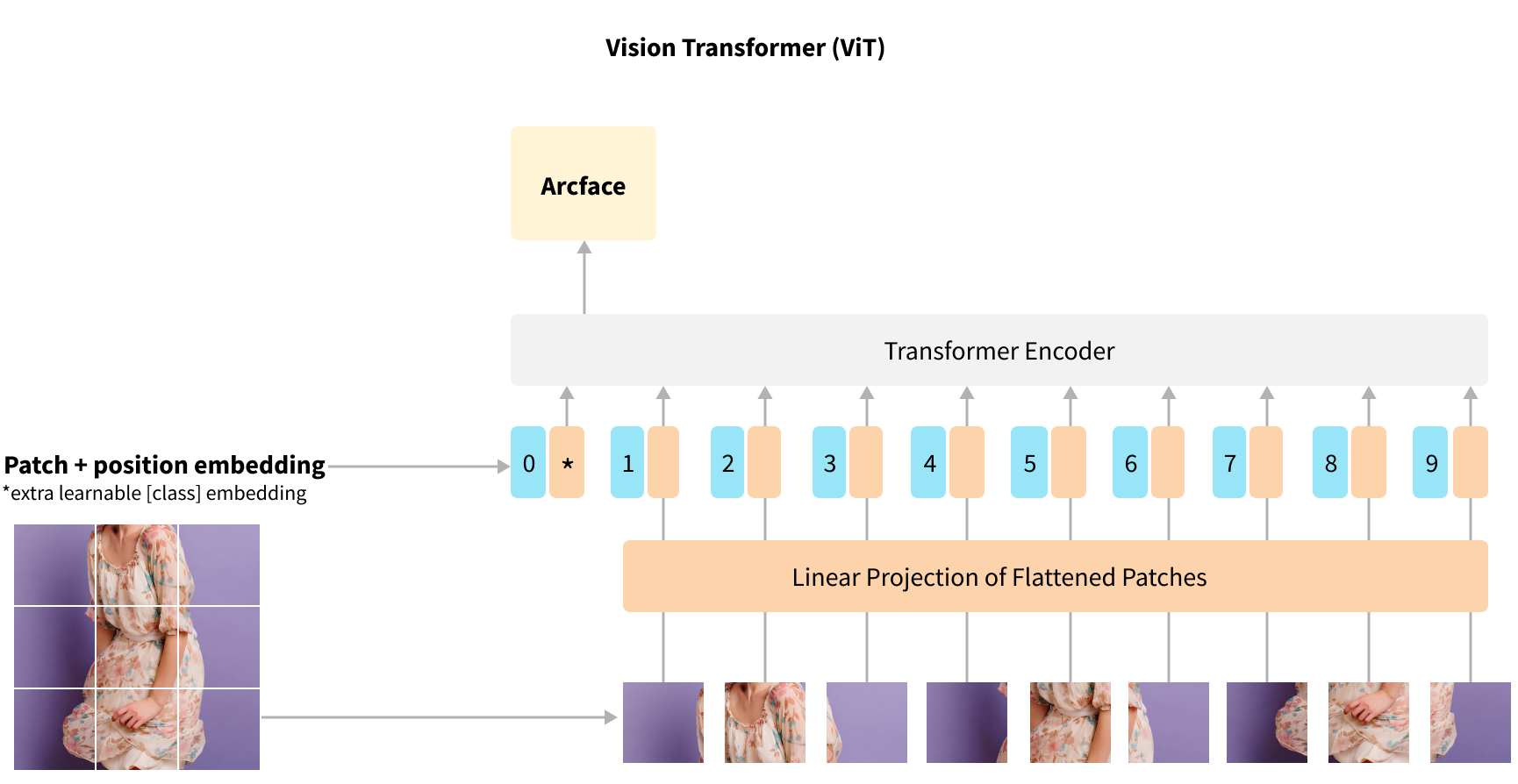
Vision transformer extends the common transformer approach by creating a sequence of 16x16 image patches from the original image. The patches are embedded using a fully connected layer, a special CLS token is prepended to the sequence and positional encoding is summed into each patch. The resulting tensor is passed first into a standard Transformer block and then to a classification head.
Model performance optimizations
The most straightforward approach to further enhance the model quality is to increase the image resolution. DeiT backbone supports 384x38 resolution, so we conducted our experiments with that resolution. This improved our scores by 3% (16% of error) but slowed down our training process by roughly 3 times. So, we continued our experiments on smaller resolutions reserving higher resolution models for production.
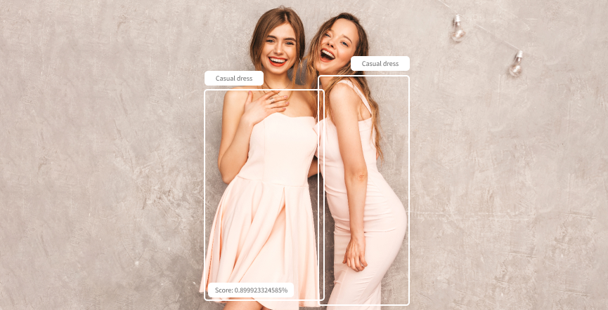
To further improve the model quality we added object detection to the model training pipeline. We leveraged the original street2shop dataset which contained bounding boxes to train the YOLOv5 object detection model. Applying this model will focus search on the apparel itself ignoring background noise. After such a model is trained we add one more preprocessing step into our training pipeline. For each image we run object detection and use a bounding box patch with a corresponding label instead of the original image. Sometimes object detection returns multiple boxes with the same label or not returns any label of proper type. In the first case, we are using the most confident one. In the second scenario we are just using the original image.
As our model has to find similar clothes within various product types (such as dresses, tops, pants, etc.), we need to ensure that model does not mix the product types. To achieve this, we modified our model architecture to add additional product type classification loss. Thus, our final loss summed up ArcFace loss and classification Cross-Entropy loss.
We experimented with two configurations for additional product type loss. In the first approach, we added a fully-connected layer on top of feature's generation layer in our network, so product type classification gradients back-propagate through the whole network, including a layer with the final embeddings used by KNN. The second approach was inspired by the GrokNet paper. Instead of sending gradients through our item embeddings, we added a secondary fully-connected classification layer on top of the final layer in the backbone network.
The first approach showed better results: as we observed the improvement in the quality metrics and manual results assessment.
Results
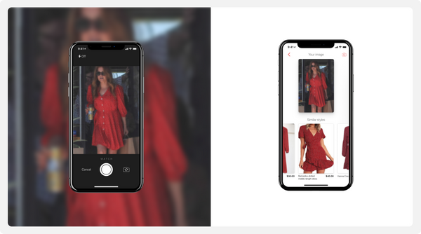
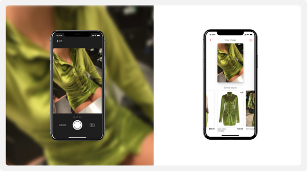
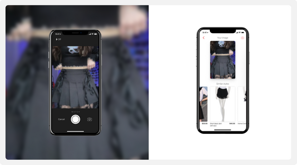
As a result, our visual search model can reliably detect and match catalog products, even in casual street images:
As a nice side effect, the item embeddings obtained with our visual model can be reused downstream in a variety of systems, such as recommenders and semantic vector search.
Conclusion
In this blog post, we shared our experience building the Street-to-Shop visual search system, from data gathering and cleansing to model design, training and evaluation.
As with many deep learning projects, a large, diverse and clean dataset is a key factor in the project’s success. However, even if you don't have such a dataset yet, don't hesitate - there are a lot of sources to obtain, mine, crawl and clean necessary data.
Modern image processing models and training algorithms allow you to achieve great results even with modest datasets.
Hope you enjoyed this dive into the street-to-shop model. If you have questions or would like to learn how Grid Dynamics can help you create a best-in-class visual search experience, don't hesitate to reach out. Happy searching!
