Xgboost vs Catboost vs Lightgbm: which is best for price prediction?
The promotions manager couldn’t believe it. For weeks, he had carefully planned the promotion, running the numbers again every day just to double check that everything made fiscal sense. By all indications, the promotion would increase demand and be a big money maker for the company, so he was excited to see the end results.
And yet, a few days into the campaign, something was not right. The financial reports showed that because of the campaign, overall revenues were up. However, when looking at the profit margins, all he saw was red. Many of the SKUs in the promotion had also been applied to other discount campaigns. The promotions manager hadn’t been aware of this overlap that had allowed many items to have been sold below their margins, costing the company money. A lot of money.
This was the situation that one of our retail customers found themselves in, unknowingly losing money when it ran certain promotions that it had expected to be very successful. The reason for this was that savvy customers were taking advantage of other concurrently running promotions. These shoppers had worked out that they could combine several different older promotional offers to receive huge discounts. The end result was that our retail customer was actually selling items far below the expected sales price at very low or even negative margins.
The retail customer approached our team with the hope that we could find a technological solution to the problem. After looking at the issue in more detail, we developed an idea. By leveraging our customer's online sales data, we created a machine learning model that could feed in key information such as historical sales and promotion data to predict the expected profit for a given product price range. Based on that prediction, we could then see which items were at risk of being sold below margins, and optimize prices accordingly.
The prediction engine would be paired with the development of a warning system that would automatically notify our customer of the highest risk items in the range. Based on those warnings, the customer could then tweak their planned promotions to mitigate any potential losses caused by selling products at low or negative margins while still being able to develop successful promotions that would continue to attract shoppers. The only question then was “how to go about building the best model”.
Which algorithm to choose?
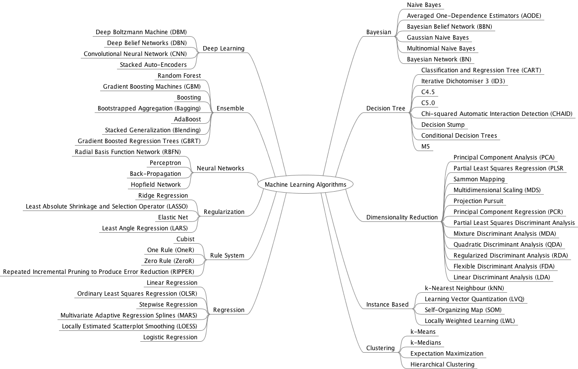
Coming up with the idea to utilize machine learning was the easy part. The hard part was deciding which algorithm/implementation to use. Due to the plethora of academic and corporate research in machine learning, there are a variety of algorithms (gradient boosted trees, decision trees, linear regression, neural networks) as well as implementations (sklearn, h2o, xgboost vs lightgbm vs catboost, tensorflow) that can be used. This means that our team has a multitude of tools available to develop a predictive model, but no existing guidelines that detail which algorithms or implementations are best suited to different types of use cases.
 Image source: Choices galore for ML algorithms (https://jixta.wordpress.com/2015/07/17/machine-learning-algorithms-mindmap/)
The potential models that our team investigated included model stacking, linear regression, decision trees, deep learning (specifically Long Short Term Memory), and gradient boosted trees.
The following provides a summary of each of the models including various features, strengths, and weaknesses:
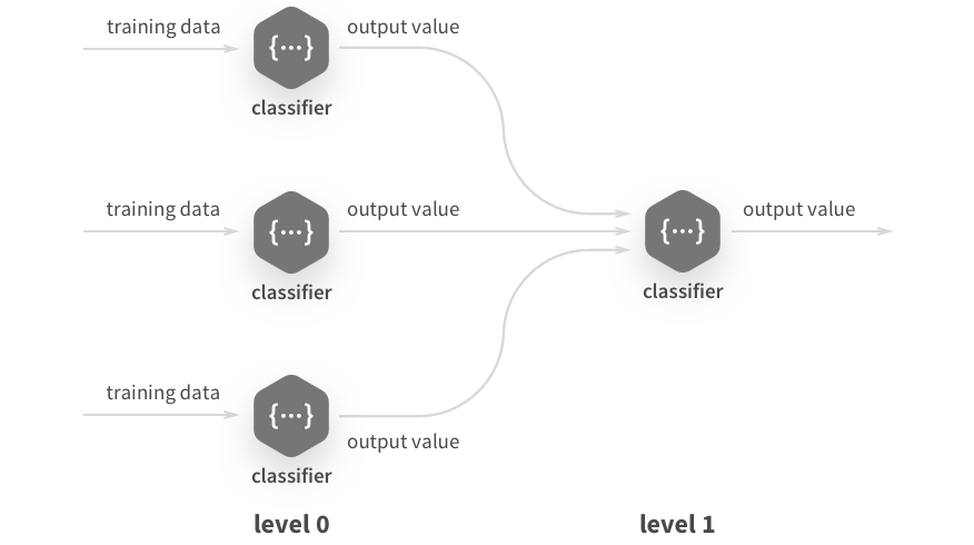
- Model Stacking: Combines the predictions of multiple models, and uses those as features for the final, predictive model
- Weaknesses: A lack of model interpretability, as well as the large amount of time needed to train multiple models, made it unfeasible for our client’s aims

- Linear Regression: Attempts to predict 'y' from our features by minimizing the sum of squared residuals
- Weakness: It makes the assumption that our features and 'y' are linearly related, which isn’t necessarily the case for sequential time-series data. This means that there's a high probability of the predictions being inaccurate
- Decision trees: Develops predictions of 'y' based on ‘rules’ or ‘decisions’ of our features
- Weakness: The fact that the algorithm is limited to one tree curbs its predictive power, and can result in inaccuracies
- LSTM: Uses a combination of memory gates and ‘neurons’ in our hidden layer(s) to help develop predictions of 'y' from our feature set
- Weaknesses: Deep learning requires by far the most computational resources, and lacks any semblance of model interpretability, making it poorly suited for our task
- Gradient Boosted Trees: Aggregates a group of small decision trees and uses that to predict 'y' from our features
- Weaknesses: Model interpretability is worse than decision trees, and it’s the third most computationally intensive algorithm after model stacking and LSTMs
Additionally, our team investigated Kaggle competitions that involved predicting future prices/sales. We noticed that the winning competitions almost always used gradient boosted trees as their algorithm of choice. Based on those findings, our team decided to utilize gradient boosted trees.
While we considered using combinations of gradient boosted implementations (as many Kaggle users had done), this approach had a couple problems that would’ve made it tricky. The first issue was the way the implementations grew and pruned their trees differed from one another. This meant we couldn’t simply re-use code for xgboost, and plug-in lightgbm or catboost. Instead, we would have to redesign it to account for different hyper-parameters, as well as their different ways of storing data (xgboost uses DMatrix, lightgbm uses Dataset, while Catboost uses Pool).
The second issue was that our client needed predictions in a timely fashion, and running multiple models would run counter to that. Figuring that it would be too much work for very little gain to incorporate all three, our team then looked into figuring out which of the three implementations we should dedicate to using.
While our hope was that there would be clear guidelines available to assist in determining which of the three to use, that wasn’t the case. Kaggle users showed no clear preference towards any of the three implementations. Additionally, tests of the implementations’ efficacy had clear biases in play, such as Yandex’s catboost vs lightgbm vs xgboost tests showing catboost outperforming both. Thus, we needed to develop our own tests to determine which implementation would work best.
Determining the best gradient boosted tree implementation ourselves
With no clear preferred implementation option, our team decided to develop our own tests. Since this was the pre-production stage, our client hadn’t provided us with any test data. We therefore needed to find our own to try and ‘simulate’ model performance. Additionally, since our problem involved price prediction, we needed to find data that was both time-series dependent, as well as involved in price prediction in some capacity. One dataset that fit very well was the Rossman dataset, as it also involved promotions data.
Once we found the data, the next step involved evaluating performance. However, there was one big problem. As mentioned above, xgboost, lightgbm, and catboost all grow and prune their trees differently. Thus, certain hyper-parameters found in one implementation would either be non-existent (such as xgboost’s min_child_weight, which is not found in catboost or lightgbm) or have different limitations (such as catboost’s depth being restricted to between 1 and 16, while xgboost and lightgbm have no such restrictions for max_depth).
Eventually, we decided on a certain subset of hyper-parameters, ones that were found on all three implementations:
- Number of trees/iterations/estimators to be grown
- Max depth (with each being restricted to between 1 and 16)
- Learning rate
These were used for GridSearchCV and RandomizedSearchCV. For early stopping, we created a model with all of the default parameters, except for number of trees/iterations/estimators. These we set to 9,999, so that we could get a good idea of the number of trees needed until overfit, as well as the time taken.
We additionally encountered a bug with catboost regarding GridSearchCV and RandomizedSearchCV: it crashed the python kernel when initializing n_jobs to be anything other than 1. So, current results do not take into account either parallelization or GPU training due to Intel GPU set-up.
We divided the dataset into train and test sets, with the training set being all data from 2014, while the test set involved all data from 2015. From there we tested xgboost vs lightgbm vs catboost in terms of speed and accuracy. This was done by utilizing sklearn’s RandomizedSearchCV and GridSearchCV, with TimeSeriesSplit as the cross-validator for each, as well as early stopping.
Results
| Implementation | GridSearch CV time | GridSearch CV RMSE | Randomized SearchCV time | Randomized SearchCV RMSE | Early stopping time | Early stopping RMSE |
| xgboost | 2064 s | 478.03 | 1488 s | 485.39 | 205 s | 480.588 |
| lightgbm | 240 s | 774.08 | 102 s | 643.38 | 74 s | 475.219 |
| catboost | 1908 s | 2993.34 | 540 s | 731.29 | 453 s | 582.82 |
As the table above demonstrates in lightgbm vs xgboost vs catboost, lightgbm was the clear winner in terms of speed, consistently outperforming catboost and xgboost. In terms of model accuracy, xgboost was the clear winner in both GridSearchCV and RandomizedSearchCV, with the lowest root mean squared error. For early stopping, lightgbm was the winner, with a slightly lower root mean squared error than xgboost.
Overall, catboost was the obvious underperformer, with training times comparable to xgboost, while having the worst predictions in terms of root mean squared error.
Based on these results, we were able to develop two general paths when deciding which implementation to use:
Path one - If you prioritize speed over accuracy (such as wanting to develop predictions as quickly as possible or wanting to test many different models), lightgbm is the algorithm of choice.
Path two - If you prioritize accuracy over speed, xgboost is the algorithm of choice.
For our project, since our retail customer wanted to minimize the instances of false negatives (reporting that a promotion would cause certain items to be sold at a loss when that wasn’t the case), we focused on emphasizing accurate predictions. Hence, we selected xgboost.
Conclusion
The rapid advances in big data and machine learning have given many industries new ways of engaging and solving customer-related problems. However, this speed of adoption has not been accompanied by the development of clear guidelines, leading to ambiguity in regards to knowing which algorithms and implementations to use for given issues.
This is not a problem that is unique to any single business or industry; it can be found in retail, healthcare, finance and even tech. Because of this, our approach of testing certain implementations of gradient boosted trees and establishing clear guidelines for usage can be applied to any company looking to use machine learning to solve a problem. This process allows companies that don't know where to start or which algorithm/implementation to use, to reduce pre-production time from a matter of days to hours or even minutes.
Conor McNamara
